Understanding Linear Regression in R

Linear Regression deals with gathering the output of a dependent variable by evaluating how the independent variable is behaving under similar circumstances. Linear regression is based on the straight line equation which is y = mx+c. Here, y is the dependent variable and x is the independent variable.

Linear Regression is based on Ordinary Least Square Regression. It is important to know the following types of variables as well:

Dependent Variable – A Dependent Variable is the variable to be predicted or explained in a regression model. This variable is assumed to be functionally related to the independent variable.

Independent Variable – An Independent Variable is the variable related to the dependent variable in a regression equation. The independent variable is used in a regression model to estimate the value of the dependent variable.

For example, we take two kinds of variables such as amount of rainfall and wheat production. The wheat production variable is the dependent variable and the amount of rainfall is the independent variable. There can also be more than one independent variable. When there is just one independent variable it is called Simple Linear Regression. If there is more than one variable it is called Multiple Linear Regression.

Let us take a case where a professor is trying to show his students the importance of mid-term test. He believes that higher the grade for mid-term, higher the final grade. A random sample of 15 students in his class was selected with a data that includes their mid-term grade and final grade.

The assumption being higher the grade for mid-term would result in a higher grade for final-term.

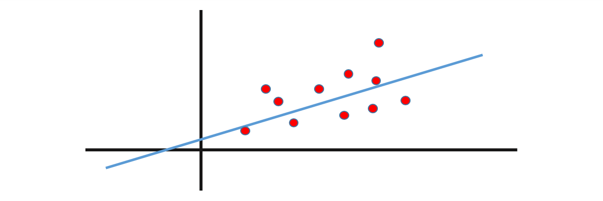
A scatter plot is created using the final grade and mid-term grade variables. If the user needs to predict the final grade based on the strengths of the mid-terms grade in the next session, he can design a linear regression model on the previous data.

We always put dependent variable on Y-axis and independent variable on X-axis.

There is a positive correlation here. Regression is a further step of correlation. If two items are correlated and we wish to find a mathematical equation for them then we use regression.

The Curvilinear (Negative Slope) denotes that two variables don’t have to necessarily be associated with each other and can have a non-linear relationship. The no relationship graph shows when variable are not correlated. The assumption for developing a linear regression model:

1. The variables must have a linear relation
2. If the data is huge and we use R, there should be a way to reject/accept the model for prediction.

The Types of Linear Relationships are:

Positive Linear Relationship – it shows the positive relationship between two variables.

Relationship NOT  Linear – There is a relationship where we can put the points in a mathematical equation.

Negative Linear Relationship – It shows the negative relationship between two variables.

No Relationship – It shows that there are no relationships between two variables.

Equation for a Straight Line

We begin with the equation Y = a + b X

Y = Dependent variable

A = Y-intercept

B = Slope of the line

X = Independent variable

Y & X are linearly independent and linearly correlated with high correlation. A & B are constant terms and there are no exponential signs in the equation.

In the multiple regression model, there are multiple x in the form of x1, x2, x3 and so on.

Intercept – When we draw a line through the Y-axis and the distance between the regression line and Y axis is called the Intercept.

Slope of the Line – It is the angle between the Regression line and the X-Axis is the Slope of the Line.

Let us take a case of Simple Linear Regression where we need to examine the linear dependency of the annual sales of grocery stores on their sizes in square footage. Sample data for 7 stores is obtained with elements such as store number, square feet and annual sales.

The scatter plot denotes a positive correlation with an outlier.

 Got a question for us?? Mention them in the comments section and we will get back to you. 

Related Posts:

Business Analytics with R Training

Introduction to Business Analytics with R