Mastering Excel Formulas: Essential Functions for Every Spreadsheet User

All of us have used an Excel sheet at least once because it has been around for a while. However, Excel is a very good program that is very compatible and flexible. Many organizations use it extensively for data processing, analysis, and recording. The Excel Formula/ Functions feature is one of the most fundamental and frequently utilized ones in Excel, Additionally, these Excel formulas should be known by all Excel users. 

We’ll take you step-by-step through several of these crucial formulas in this blog. Along the way, we’ll offer helpful hints and strategies for Excel that will make learning more dynamic and interesting. By the time it’s through, you’ll know a lot about Excel formulas and be prepared to take on any data challenge that comes your way.

Now, let’s get started and utilize Excel formulas to their fullest potential. Prepare to astound your coworkers, increase your output, and quickly become an Excel pro!

Table of Contents

• What Is Excel Formula?
• Why Is It Important to Know These MS Excel Formulas?
• The Benefits of Learning Excel Formulas
• TOP 20 Formulas in Excel
• Conclusion
• FAQs
  • Which Excel formulas are fundamental?
  • Is there a need for Excel specialists?
  • What are the functions and formulas in MS Excel?
  • What are the fundamentals of Excel?
  • Which five Excel formulas are essential?

What Is Excel Formula?

An expression that works with values in a range of cells is called a formula in Microsoft Excel. Even when a result is incorrect, these formulas still return a result. You can carry out operations like addition, subtraction, multiplication, and division using Excel formulas. In addition to these, you can work with date and time values, compute percentages and averages for a range of cells in Excel, and much more.

Although these two terms are frequently used synonymously, technically speaking, it is nothing but a Formula: the equation that the user manually enters.

Now that you have a clear picture of what Excel is, let us look at why it is important to know these MS Excel formulas.

Why Is It Important to Know These MS Excel Formulas?

If you have the right training and skill set, you might be a talented worker who is prepared to take on challenges at work. But what distinguishes you from the rest of the pack? Why does the employer want you to stay on? It takes more than just hard work, though; you also need to be an intelligent worker with the fundamental skill sets required for daily tasks.

Almost all businesses use Microsoft Excel for a wide range of tasks, including data analysis, data storage, strategic analysis, report generation, and much more. Additionally, learning the fundamentals of Excel is required of everyone. Excel formulas are one of the many features available in Excel spreadsheets. 

Now we’ll discuss the advantages of learning Excel formulas.

The Benefits of Learning Excel Formulas

Is it worth the time for people who are considering learning Excel formulas? In a recent survey, more than 90% of workers said that they depend on Excel formulas for their jobs.

Top 5 Benefits of Learning Excel Formulas: – 

• It simplifies your work.
• Developing your skill sets is always a plus.
• More adept at data organization.
• Making you an invaluable worker for the business.
• Boosts production and efficiency. 

Now we will move on to the main part, where we will discuss the top 20 Excel formulas.

TOP 20 Formulas in Excel

The following list of frequently used Excel formulas can significantly improve your skills in data analysis and manipulation:

1.Sum 

As its name implies, the SUM() function returns the sum of the values within the chosen range of cells. It executes addition, a mathematical operation. Below is an example of it:

SUM =SUM(C3:C5)

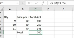As you can see above, all we had to do was enter the function “=SUM(C3:C5)” to determine the total amount for each unit. 105, 250, and 345 automatically add up to this. The outcome is kept in C6.

2 . Percentage 

You can use Excel’s built-in PERCENTAGE function or basic arithmetic operations to compute a percentage.

Percentage =B2/B3

I will add two random numbers, 5 and 8, to the percentage value calculation; 5(B2) is the path value and 8(B3) is the total value. After choosing the cell(B4)l in which you want the result to appear when you type the (= ) symbol, choose the value, and divide it. 

3 . IF 

Excel’s IF function allows you to perform conditional logic, which means you can specify different actions based on whether or not a specific condition is met.

If a condition is TRUE, the IF() function evaluates it and returns a specific value. If the condition is FALSE, it will return a different value.

IF =IF(A2>8,”YES”,”NO”)

We wish to determine whether the value in cell A2 in the example below is greater than 8. The function will return “Yes, four is greater” if it is greater than 8; otherwise, it will return “No.”

Since four is not greater than 8, it will return “No” in this instance.

4 . Average 

Excel has a built-in function for average, which is one of the simplest methods.

The AVERAGE function is commonly used in Excel to calculate averages such as test scores, sales figures, and temperatures. It is an essential tool for data analysis and reporting.

As demonstrated by the example below, all you have to do to find the average of the total sales is type in:

Average =Average(E5,E6)

The average is computed automatically, and you can store the outcome where you’d like.

5 . Count

The total number of cells in a range containing a number is counted by the function COUNT(). The blank cell and the cells containing data in any format other than numeric are excluded.

COUNT =COUNT(B3:B5)

We are counting from B2 to B5, ideally four cells, as can be seen above. The cell containing “TEST marks” is omitted in this case, so the answer is three since the COUNT function only considers cells with numerical values. 

6. CountA

Excel’s COUNTA function counts the number of cells in a range that are not empty. Any kind of data, including text, numbers, logical values, errors, and empty strings, are counted in the cells.

COUNTA =COUNTA(B2:B6)

From A2 to A6, as shown in A7, you can observe that there are four non-empty cells. Similarly, from B2 to B6, there are three non-empty cells, as shown in B7. 

7. COUNTIF 

Excel’s COUNTIF function counts the number of cells in a range that satisfy a given requirement. With it, you can set a criterion and then determine how many cells in the range satisfy it.

Range: This is the collection of cells to which the criteria are to be applied.

These are the requirements or standards that you wish to apply to the range. It might be an expression, a text, a number, or a link to a cell that contains a value.

COUNTIF =COUNTIF(A2:D2,”>70”)

In the example above, I’ve entered the scores from tests 1, 2, and 3, along with the condition that the marks must be greater than 70. Using the countif Formula, I was able to determine the answer, which was 5

8. Index

The value of a cell in a given row and column of a range is returned by Excel’s INDEX function. When obtaining data from tables or arrays, it is very helpful.

Array: This is a representation of the range or array from which a value is to be obtained.

row_num: The array’s row number from which you want to get a value is indicated here.

column_num (optional): This is the array’s column number that you wish to retrieve a value from. INDEX returns the value of the entire row indicated by row_num if it is omitted. 

INDEX =INDEX(A2:D5,3,3)

In the example above, I will be utilizing the INDEX formula. I have selected the array A2 to D5, assigned a row value of 3, a column value of 3, and an index value of 78. 

9 . Finding the grade 

Use Excel’s IF function to apply different conditions and return the appropriate grade in order to determine the grade based on a score. 

Based on the given conditions, this Formula assesses each score in column A and determines the appropriate grade. It returns “A” if the score is greater than or equal to 70. If not, it ascertains whether the score is forty or higher, and so forth. It returns a “F” if none of the requirements are met.

=IF(B2>70,”A”,IF(B2>40,”B”,”F”))

10 . LEN

Excel’s LEN function counts the characters in a given text string. Figuring out the length of text, including spaces and markup, is very helpful. 

Text: This is the text string that you want the character count for.

Here’s an illustration of how to utilize the LEN function.

LEN =LEN(A2)

HELLO, WORLD 

This Formula will return the number of characters in the text string “Hello, World!” which is 12 characters.

11. SUMIF

Excel’s SUMIF function is used to total the values within a range that satisfies certain requirements. You can specify the range of values to sum, the criteria to apply, and the range to evaluate. 

Range: The cells you wish to compare to the criteria fall within this range.

Criteria: This is the requirement or standard that you plan to use with the range. It could be a text string, an expression, or a number.

sum_range (optional): This is the cell range that your values should be added to. Excel will use the range for adding and evaluating criteria if it is left out.

SUMIF  =SUMIF(A3:A6,A6,B3:B6)

When we added the values for sum_range, which is HONDA, in the example above, we got 666 as the result.

12 . LEFT 

Excel’s LEFT function pulls a predetermined number of characters from a text string’s left side. It’s very helpful for eliminating certain characters from text strings, such as IDs, codes, and names.

Text: The text string you want to extract characters from is this one.

Character count (optional): Indicates how many characters you want to take out of the text string’s left side. Excel will automatically extract the first character if it is left out.

LEFT  =LEFT(B3,3)

The B3 character has been designated as the “text” in the example above, and the number of characters to be extracted is 3. 

13 . RIGHT

Excel’s RIGHT function pulls a predetermined number of characters from a text string’s right side. It is particularly useful for extracting characters from text strings, such as IDs, codes, and file extensions.

RIGHT  =RIGHT(B3,2)

The “text” in the example above has been designated as the B3 character, and there are 2 characters that need to be extracted. 

14 . TRIM

Excel’s TRIM function eliminates extra spaces from text, leaving only single spaces—neither leading nor trailing—between words. Because it cleans and standardizes text data, it’s especially helpful when working with text that has been imported from other sources. 

Text: This is the text string that needs to have any extra spaces removed.

TRIM  =TRIM(A1)

In the example above, we are using the trim Formula to eliminate the extra space between HOW IS THE CAT

15 . MIN

Excel’s MIN function can be used to determine the lowest value within a range of cells or a list of numbers. Within the given range, it returns the lowest value. 

These are the numbers, cell references, or ranges that you want to take the minimum value from, starting with number one, number two, etc. Up to 255 distinct values, ranges, or cell references can be specified.

MIN  =MIN(B2:B4)

We have included the names of the students and their marks in the Excel sheet. We will then utilize the min formula to determine the minimum marks that were earned. 

16 . MAX

Excel’s MAX function can be used to determine the maximum value within a range of cells or a group of numbers. It gives back the highest value that falls inside the given range.

MAX  =MAX(B2:B4)

In the Excel sheet, we have listed the students’ names and marks. Next, we’ll apply the MAX formula to ascertain the student’s maximum marks achieved. 

17 . CONCATENATE 

Multiple strings or cell values can be concatenated into a single string using Excel’s CONCATENATE function. It is particularly helpful for generating dynamic text strings and merging text strings, like last and first names. 

CONCAT  =CONCAT(A2:B5)

The concat Formula is used in the example above to combine or concatenate multiple strings or cell values into a single string that runs from A2 to B5.

18 . HLookup

The HLOOKUP function in Excel retrieves the value from the designated row after searching for it in the top row of a table or range of cells. It is the VLOOKUP function in a horizontal format.

Lookup_value: This is the value that you should look up in the top row of the table.

table_array: The range of cells that comprise the table is indicated here. The values to be searched are in the first row of this range, and the data to be returned is in the rows that follow.

row_index_num: This is the table_array row number that you want to get data from. The table_array’s first row of data has a number in it.

Range lookup (not required): Whether you want an exact match or an approximation is indicated by this argument. It may accept any of the subsequent values

A rough match is indicated by TRUE or 1, which is the default. The closest match that is less than or equal to the lookup_value is returned if an exact match cannot be found.

0 or FALSE: Perfect match. If there isn’t a precise match, an error is returned.

HLOOKUP  =HLOOKUP(A1,A1:C4,2,FALSE)

In the example above, we have classified a single person’s name, email address, and salary using the HLOOKUP formula. The HLOOKUP value represents the name you wish to add, the table array represents the entry table, and the row number, which is 2, is indicated by the row index number. False is the range lookup. 

19 . VLOOKUP

The VLOOKUP function in Excel retrieves a value from the designated column in the same row after searching for a value in the first column of a table or range of cells. It’s among Excel’s most often used vertical lookup functions.

lookup_value: This is the value that you should look for in the first column of the table.

Table array: The range of cells that comprise the table is this. The values to be searched are listed in the first column of this range, and the data to be returned is listed in the subsequent columns.

col_index_num: This is the table_array column number that you want to retrieve data from. The number one appears in the table_array’s first column of data.

Range lookup (optional): This parameter lets you specify if you’re looking for an exact or approximate match.

VLOOKUP  =VLOOKUP(A3,A1:C4,1,FALSE)

The VLOOKUP formula was used in the example above to classify the name, email address, and salary of a single individual. The table array represents the entry table, the COLUMN index number indicates the COLUMN number, which is 1, and the VLOOKUP value represents the name you want to add. This range lookup is false. 

20 . Date/day

The DATE function can be used to generate a date from its components (year, month, and day).

Year: The year in which the date occurred.

Month: The month in which the date falls (1 for January, 2 for February, etc.).

Day: The current date.

All three of the parameters—Year, Month, and Day—in the example above are necessary and mandatory. The Year, Month, and Day that are enclosed in parentheses should be replaced with cell references. It will retrieve values in the format of a date from those cells. 

DATE  =DATE(23,4,8)

Conclusion

Excel is a very strong spreadsheet program for reporting and data analysis. You should have gained knowledge of the key Excel functions and formulas after reading this article, which will enable you to complete your work more quickly and effectively. We examined advanced Excel formulas and functions as well as text and numeric. It goes without saying that proficiency with Excel greatly influences many career paths.

These are some of the frequently asked questions.

FAQs

1. Which Excel formulas are fundamental?

Arithmetic operations such as addition, subtraction, multiplication, and division—for instance, SUM, AVERAGE, COUNT, and PRODUCT—are included in Excel’s basic formulas.

2. Is there a need for Excel specialists?

Because MS Excel is used extensively in many different industries, there is a great need for people with advanced skills in the program.

3. What are the functions and formulas in MS Excel?

Formulas and functions in Microsoft Excel are expressions that are used to carry out calculations or work with data. Formulas can include functions, mathematical operations, cell references, and constants. They begin with the equal sign (=).

4. What are the fundamentals of Excel?

Data entry is one of the fundamental Excel skills.

• Cell formatting.
• Using fundamental functions and formulas.
• Making easy charts.
• Data filtering and sorting.
• Recognizing references in cells.

5. Which five Excel formulas are essential?

Several crucial Excel formulas are as follows:

• SUM: A range of cell values are added using the SUM formula.
• AVERAGE: The values in a range of cells are averaged using the AVERAGE Formula.
• COUNT: The COUNT formula determines how many cells within a specified range of cells contain numeric values.
• IF: The IF formula evaluates a condition, and if it is true, it returns a particular output; if it is false, it returns a different result.
• VLOOKUP: This Formula looks up a value in a table and returns the value that corresponds to that value in a different table column.

Enroll in Edureka’s Advanced MS Excel 2016 Certification Training if you want to progress your career.

All jobs in the analytics and consulting industry will require the knowledge you will acquire. This course will teach you the advanced functions that analysts use on a daily basis. Additionally, you’ll become used to even more sophisticated Excel functions, such as macros, which are very helpful. You will be given practical assignments and case studies throughout the course to apply the theoretical knowledge. To further your career, enrol immediately! Take action right now!

Have a query for us? Kindly let us know in the comments section, and we’ll get in touch with you.