Full Stack Web Development Internship Program
- 29k Enrolled Learners
- Weekend/Weekday
- Live Class
(11250)
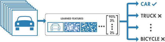
Image Classification a task which even a baby can do in seconds, but for a machine, it has been a tough task until the recent advancements in Artificial Intelligence and Deep Learning. Self-driving cars can detect objects and take required action in real-time and most of this is possible because of TensorFlow Image Classification. In this article, I’ll guide you through the following topics:
TensorFlow is Google’s Open Source Machine Learning Framework for dataflow programming across a range of tasks. Nodes in the graph represent mathematical operations, while the graph edges represent the multi-dimensional data arrays communicated between them.
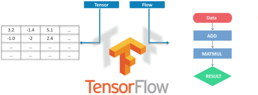
Tensors are just multidimensional arrays, an extension of 2-dimensional tables to data with a higher dimension. There are many features of Tensorflow which makes it appropriate for Deep Learning and it’s core open source library helps you develop and train ML models.
The intent of Image Classification is to categorize all pixels in a digital image into one of several land cover classes or themes. This categorized data may then be used to produce thematic maps of the land cover present in an image.
Now Depending on the interaction between the analyst and the computer during classification, there are two types of classification:
So, without wasting any time let’s jump into TensorFlow Image Classification. I have 2 examples: easy and difficult. Let’s proceed with the easy one.
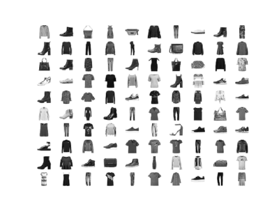
Fashion MNIST Dataset
Here we are going to use Fashion MNIST Dataset, which contains 70,000 grayscale images in 10 categories. We will use 60000 for training and the rest 10000 for testing purposes. You can access the Fashion MNIST directly from TensorFlow, just import and load the data.
from __future__ import absolute_import, division, print_function
# TensorFlow and tf.keras

import tensorflow as tf
from tensorflow import keras

# Helper libraries

import numpy as np
import matplotlib.pyplot as plt
fashion_mnist = keras.datasets.fashion_mnist

(train_images, train_labels), (test_images, test_labels) = fashion_mnist.load_data()
class_names = ['T-shirt/top', 'Trouser', 'Pullover', 'Dress', 'Coat','Sandal', 'Shirt', 'Sneaker', 'Bag', 'Ankle boot']
train_images.shape
#Each Label is between 0-9
train_labels
test_images.shape
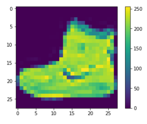
plt.figure()
plt.imshow(train_images[0])
plt.colorbar()
plt.grid(False)
plt.show()
#If you inspect the first image in the training set, you will see that the pixel values fall in the range of 0 to 255.
train_images = train_images / 255.0

test_images = test_images / 255.0
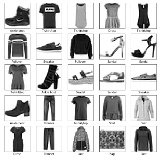
plt.figure(figsize=(10,10))
for i in range(25):
    plt.subplot(5,5,i+1)
    plt.xticks([])
    plt.yticks([])
    plt.grid(False)
    plt.imshow(train_images[i], cmap=plt.cm.binary)
    plt.xlabel(class_names[train_labels[i]])
plt.show()
model = keras.Sequential([
    keras.layers.Flatten(input_shape=(28, 28)),
    keras.layers.Dense(128, activation=tf.nn.relu),
    keras.layers.Dense(10, activation=tf.nn.softmax)
])
model.compile(optimizer='adam',
              loss='sparse_categorical_crossentropy',
              metrics=['accuracy'])
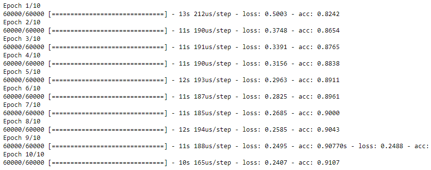
model.fit(train_images, train_labels, epochs=10)
test_loss, test_acc = model.evaluate(test_images, test_labels)

print('Test accuracy:', test_acc)
![]()
predictions = model.predict(test_images)
predictions[0]
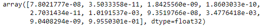
A prediction is an array of 10 numbers. These describe the “confidence” of the model that the image corresponds to each of the 10 different articles of clothing. We can see which label has the highest confidence value.
np.argmax(predictions[0])
#Model is most confident that it's an ankle boot. Let's see if it's correct
Output: 9
test_labels[0]
Output: 9
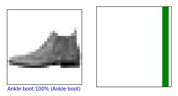
def plot_image(i, predictions_array, true_label, img):
  predictions_array, true_label, img = predictions_array[i], true_label[i], img[i]
  plt.grid(False)
  plt.xticks([])
  plt.yticks([])

  plt.imshow(img, cmap=plt.cm.binary)

  predicted_label = np.argmax(predictions_array)
  if predicted_label == true_label:
    color = 'green'
  else:
    color = 'red'

  plt.xlabel("{} {:2.0f}% ({})".format(class_names[predicted_label],
                                100*np.max(predictions_array),
                                class_names[true_label]),
                                color=color)

def plot_value_array(i, predictions_array, true_label):
  predictions_array, true_label = predictions_array[i], true_label[i]
  plt.grid(False)
  plt.xticks([])
  plt.yticks([])
  thisplot = plt.bar(range(10), predictions_array, color="#777777")
  plt.ylim([0, 1])
  predicted_label = np.argmax(predictions_array)

  thisplot[predicted_label].set_color('red')
  thisplot[true_label].set_color('green')
i = 0
plt.figure(figsize=(6,3))
plt.subplot(1,2,1)
plot_image(i, predictions, test_labels, test_images)
plt.subplot(1,2,2)
plot_value_array(i, predictions,  test_labels)
plt.show()
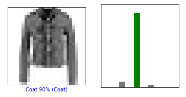
i = 10
plt.figure(figsize=(6,3))
plt.subplot(1,2,1)
plot_image(i, predictions, test_labels, test_images)
plt.subplot(1,2,2)
plot_value_array(i, predictions,  test_labels)
plt.show()
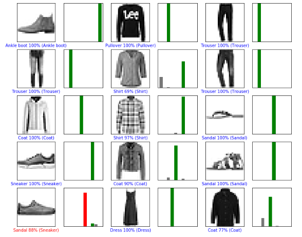
num_rows = 5
num_cols = 3
num_images = num_rows*num_cols
plt.figure(figsize=(2*2*num_cols, 2*num_rows))
for i in range(num_images):
  plt.subplot(num_rows, 2*num_cols, 2*i+1)
  plot_image(i, predictions, test_labels, test_images)
  plt.subplot(num_rows, 2*num_cols, 2*i+2)
  plot_value_array(i, predictions, test_labels)
plt.show()
# Grab an image from the test dataset
img = test_images[0]

print(img.shape)
# Add the image to a batch where it's the only member.
img = (np.expand_dims(img,0))

print(img.shape)
predictions_single = model.predict(img)
print(predictions_single)
![]()
plot_value_array(0, predictions_single, test_labels)
plt.xticks(range(10), class_names, rotation=45)
plt.show()
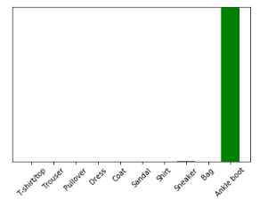
prediction_result = np.argmax(predictions_single[0])
Output: 9
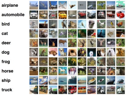
The CIFAR-10 dataset consists of airplanes, dogs, cats, and other objects. You’ll preprocess the images, then train a convolutional neural network on all the samples. The images need to be normalized and the labels need to be one-hot encoded. This use-case will surely clear your doubts about TensorFlow Image Classification.
from urllib.request import urlretrieve
from os.path import isfile, isdir
from tqdm import tqdm
import tarfile

cifar10_dataset_folder_path = 'cifar-10-batches-py'

class DownloadProgress(tqdm):
    last_block = 0

    def hook(self, block_num=1, block_size=1, total_size=None):
        self.total = total_size
        self.update((block_num - self.last_block) * block_size)
        self.last_block = block_num

"""
    check if the data (zip) file is already downloaded
    if not, download it from "https://www.cs.toronto.edu/~kriz/cifar-10-python.tar.gz" and save as cifar-10-python.tar.gz
"""
if not isfile('cifar-10-python.tar.gz'):
    with DownloadProgress(unit='B', unit_scale=True, miniters=1, desc='CIFAR-10 Dataset') as pbar:
        urlretrieve(
            'https://www.cs.toronto.edu/~kriz/cifar-10-python.tar.gz',
            'cifar-10-python.tar.gz',
            pbar.hook)

if not isdir(cifar10_dataset_folder_path):
    with tarfile.open('cifar-10-python.tar.gz') as tar:
        tar.extractall()
        tar.close()
import pickle
import numpy as np
import matplotlib.pyplot as plt
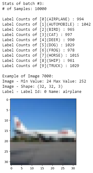
The original batch of Data is 10000×3072 tensor expressed in a numpy array, where 10000 is the number of sample data. The image is colored and of size 32×32. Feeding can be done either in a format of (width x height x num_channel) or (num_channel x width x height). Let’s define the labels.
def load_label_names():
    return ['airplane', 'automobile', 'bird', 'cat', 'deer', 'dog', 'frog', 'horse', 'ship', 'truck']
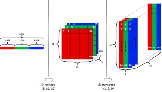
We are going to reshape the data in two stages
Firstly, divide the row vector (3072) into 3 pieces. Each piece corresponds to each channel. This results in (3 x 1024) dimension of a tensor. Then Divide the resulting tensor from the previous step with 32. 32 here means the width of an image. This results in (3x32x32).
Secondly, we have to transpose the data from (num_channel, width, height) to (width, height, num_channel). For that, we are going to use the transpose function.
def load_cfar10_batch(cifar10_dataset_folder_path, batch_id):
    with open(cifar10_dataset_folder_path + '/data_batch_' + str(batch_id), mode='rb') as file:
        # note the encoding type is 'latin1'
        batch = pickle.load(file, encoding='latin1')

    features = batch['data'].reshape((len(batch['data']), 3, 32, 32)).transpose(0, 2, 3, 1)
    labels = batch['labels']

    return features, label
def display_stats(cifar10_dataset_folder_path, batch_id, sample_id):
    features, labels = load_cfar10_batch(cifar10_dataset_folder_path, batch_id)

    if not (0 <= sample_id < len(features)):
        print('{} samples in batch {}.  {} is out of range.'.format(len(features), batch_id, sample_id))
        return None

    print('
Stats of batch #{}:'.format(batch_id))
    print('# of Samples: {}
'.format(len(features)))

    label_names = load_label_names()
    label_counts = dict(zip(*np.unique(labels, return_counts=True)))
    for key, value in label_counts.items():
        print('Label Counts of [{}]({}) : {}'.format(key, label_names[key].upper(), value))

    sample_image = features[sample_id]
    sample_label = labels[sample_id]

    print('
Example of Image {}:'.format(sample_id))
    print('Image - Min Value: {} Max Value: {}'.format(sample_image.min(), sample_image.max()))
    print('Image - Shape: {}'.format(sample_image.shape))
    print('Label - Label Id: {} Name: {}'.format(sample_label, label_names[sample_label]))

    plt.imshow(sample_image)
%matplotlib inline
%config InlineBackend.figure_format = 'retina'

import numpy as np

# Explore the dataset
batch_id = 3
sample_id = 7000
display_stats(cifar10_dataset_folder_path, batch_id, sample_id)
We are going to Normalize the data via Min-Max Normalization. This simply makes all x values to range between 0 and 1.
y = (x-min) / (max-min)
def normalize(x):
    """
        argument
            - x: input image data in numpy array [32, 32, 3]
        return
            - normalized x
    """
    min_val = np.min(x)
    max_val = np.max(x)
    x = (x-min_val) / (max_val-min_val)
    return x
def one_hot_encode(x):
    """
        argument
            - x: a list of labels
        return
            - one hot encoding matrix (number of labels, number of class)
    """
    encoded = np.zeros((len(x), 10))

    for idx, val in enumerate(x):
        encoded[idx][val] = 1

    return encoded
def _preprocess_and_save(normalize, one_hot_encode, features, labels, filename):
    features = normalize(features)
    labels = one_hot_encode(labels)

    pickle.dump((features, labels), open(filename, 'wb'))


def preprocess_and_save_data(cifar10_dataset_folder_path, normalize, one_hot_encode):
    n_batches = 5
    valid_features = []
    valid_labels = []

    for batch_i in range(1, n_batches + 1):
        features, labels = load_cfar10_batch(cifar10_dataset_folder_path, batch_i)

        # find index to be the point as validation data in the whole dataset of the batch (10%)
        index_of_validation = int(len(features) * 0.1)

        # preprocess the 90% of the whole dataset of the batch
        # - normalize the features
        # - one_hot_encode the lables
        # - save in a new file named, "preprocess_batch_" + batch_number
        # - each file for each batch
        _preprocess_and_save(normalize, one_hot_encode,
                             features[:-index_of_validation], labels[:-index_of_validation],
                             'preprocess_batch_' + str(batch_i) + '.p')

        # unlike the training dataset, validation dataset will be added through all batch dataset
        # - take 10% of the whold dataset of the batch
        # - add them into a list of
        #   - valid_features
        #   - valid_labels
        valid_features.extend(features[-index_of_validation:])
        valid_labels.extend(labels[-index_of_validation:])

    # preprocess the all stacked validation dataset
    _preprocess_and_save(normalize, one_hot_encode,
                         np.array(valid_features), np.array(valid_labels),
                         'preprocess_validation.p')

    # load the test dataset
    with open(cifar10_dataset_folder_path + '/test_batch', mode='rb') as file:
        batch = pickle.load(file, encoding='latin1')

    # preprocess the testing data
    test_features = batch['data'].reshape((len(batch['data']), 3, 32, 32)).transpose(0, 2, 3, 1)
    test_labels = batch['labels']

    # Preprocess and Save all testing data
    _preprocess_and_save(normalize, one_hot_encode,
                         np.array(test_features), np.array(test_labels),
                         'preprocess_training.p')
preprocess_and_save_data(cifar10_dataset_folder_path, normalize, one_hot_encode)
import pickle

valid_features, valid_labels = pickle.load(open('preprocess_validation.p', mode='rb'))
The entire model consists of 14 layers in total.
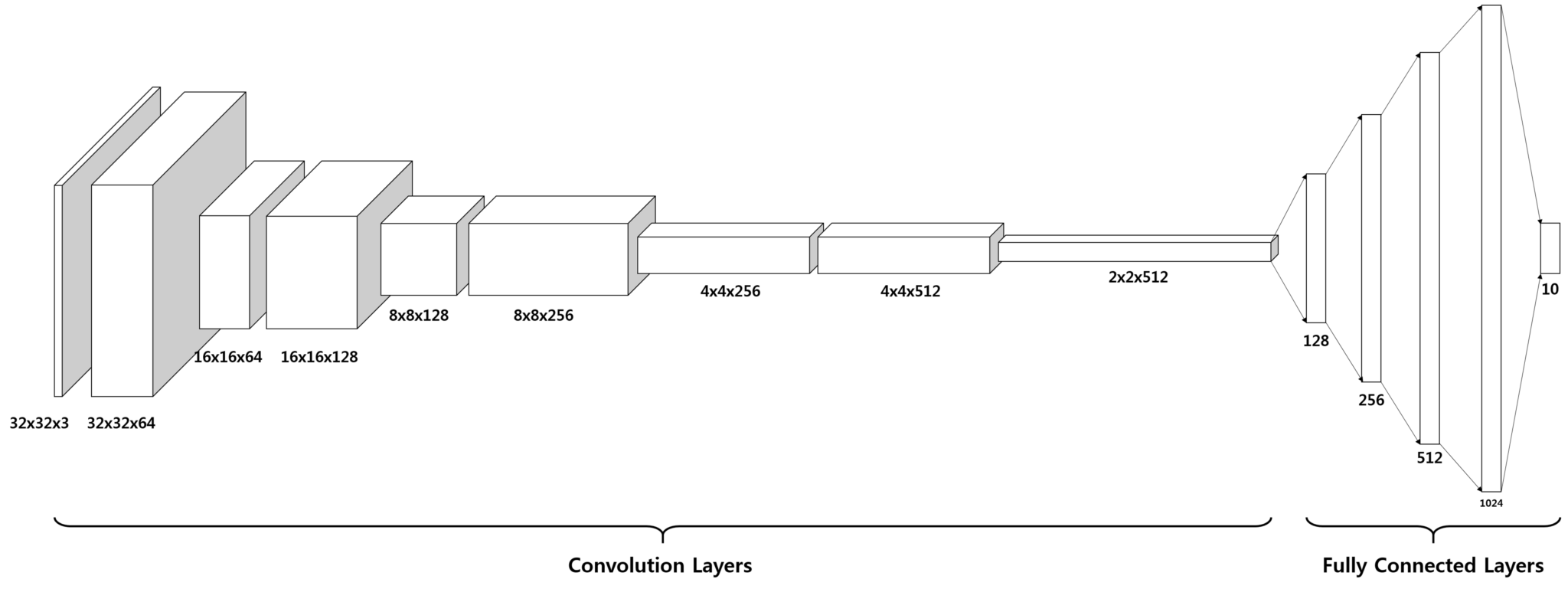
import tensorflow as tf

def conv_net(x, keep_prob):
    conv1_filter = tf.Variable(tf.truncated_normal(shape=[3, 3, 3, 64], mean=0, stddev=0.08))
    conv2_filter = tf.Variable(tf.truncated_normal(shape=[3, 3, 64, 128], mean=0, stddev=0.08))
    conv3_filter = tf.Variable(tf.truncated_normal(shape=[5, 5, 128, 256], mean=0, stddev=0.08))
    conv4_filter = tf.Variable(tf.truncated_normal(shape=[5, 5, 256, 512], mean=0, stddev=0.08))

    # 1, 2
    conv1 = tf.nn.conv2d(x, conv1_filter, strides=[1,1,1,1], padding='SAME')
    conv1 = tf.nn.relu(conv1)
    conv1_pool = tf.nn.max_pool(conv1, ksize=[1,2,2,1], strides=[1,2,2,1], padding='SAME')
    conv1_bn = tf.layers.batch_normalization(conv1_pool)

    # 3, 4
    conv2 = tf.nn.conv2d(conv1_bn, conv2_filter, strides=[1,1,1,1], padding='SAME')
    conv2 = tf.nn.relu(conv2)
    conv2_pool = tf.nn.max_pool(conv2, ksize=[1,2,2,1], strides=[1,2,2,1], padding='SAME')
    conv2_bn = tf.layers.batch_normalization(conv2_pool)

    # 5, 6
    conv3 = tf.nn.conv2d(conv2_bn, conv3_filter, strides=[1,1,1,1], padding='SAME')
    conv3 = tf.nn.relu(conv3)
    conv3_pool = tf.nn.max_pool(conv3, ksize=[1,2,2,1], strides=[1,2,2,1], padding='SAME')
    conv3_bn = tf.layers.batch_normalization(conv3_pool)

    # 7, 8
    conv4 = tf.nn.conv2d(conv3_bn, conv4_filter, strides=[1,1,1,1], padding='SAME')
    conv4 = tf.nn.relu(conv4)
    conv4_pool = tf.nn.max_pool(conv4, ksize=[1,2,2,1], strides=[1,2,2,1], padding='SAME')
    conv4_bn = tf.layers.batch_normalization(conv4_pool)

    # 9
    flat = tf.contrib.layers.flatten(conv4_bn)

    # 10
    full1 = tf.contrib.layers.fully_connected(inputs=flat, num_outputs=128, activation_fn=tf.nn.relu)
    full1 = tf.nn.dropout(full1, keep_prob)
    full1 = tf.layers.batch_normalization(full1)

    # 11
    full2 = tf.contrib.layers.fully_connected(inputs=full1, num_outputs=256, activation_fn=tf.nn.relu)
    full2 = tf.nn.dropout(full2, keep_prob)
    full2 = tf.layers.batch_normalization(full2)

    # 12
    full3 = tf.contrib.layers.fully_connected(inputs=full2, num_outputs=512, activation_fn=tf.nn.relu)
    full3 = tf.nn.dropout(full3, keep_prob)
    full3 = tf.layers.batch_normalization(full3)

    # 13
    full4 = tf.contrib.layers.fully_connected(inputs=full3, num_outputs=1024, activation_fn=tf.nn.relu)
    full4 = tf.nn.dropout(full4, keep_prob)
    full4 = tf.layers.batch_normalization(full4)

    # 14
    out = tf.contrib.layers.fully_connected(inputs=full3, num_outputs=10, activation_fn=None)
    return out
epochs = 10
batch_size = 128
keep_probability = 0.7
learning_rate = 0.001
logits = conv_net(x, keep_prob)
model = tf.identity(logits, name='logits') # Name logits Tensor, so that can be loaded from disk after training

# Loss and Optimizer
cost = tf.reduce_mean(tf.nn.softmax_cross_entropy_with_logits(logits=logits, labels=y))
optimizer = tf.train.AdamOptimizer(learning_rate=learning_rate).minimize(cost)

# Accuracy
correct_pred = tf.equal(tf.argmax(logits, 1), tf.argmax(y, 1))
accuracy = tf.reduce_mean(tf.cast(correct_pred, tf.float32), name='accuracy')
#Single Optimization
def train_neural_network(session, optimizer, keep_probability, feature_batch, label_batch):
    session.run(optimizer,
                feed_dict={
                    x: feature_batch,
                    y: label_batch,
                    keep_prob: keep_probability
                })
#Showing Stats
def print_stats(session, feature_batch, label_batch, cost, accuracy):
    loss = sess.run(cost,
                    feed_dict={
                        x: feature_batch,
                        y: label_batch,
                        keep_prob: 1.
                    })
    valid_acc = sess.run(accuracy,
                         feed_dict={
                             x: valid_features,
                             y: valid_labels,
                             keep_prob: 1.
                         })

    print('Loss: {:>10.4f} Validation Accuracy: {:.6f}'.format(loss, valid_acc))
def batch_features_labels(features, labels, batch_size):
    """
    Split features and labels into batches
    """
    for start in range(0, len(features), batch_size):
        end = min(start + batch_size, len(features))
        yield features[start:end], labels[start:end]

def load_preprocess_training_batch(batch_id, batch_size):
    """
    Load the Preprocessed Training data and return them in batches of <batch_size> or less
    """
    filename = 'preprocess_batch_' + str(batch_id) + '.p'
    features, labels = pickle.load(open(filename, mode='rb'))

    # Return the training data in batches of size <batch_size> or less
    return batch_features_labels(features, labels, batch_size)
#Saving Model and Path
save_model_path = './image_classification'

print('Training...')
with tf.Session() as sess:
    # Initializing the variables
    sess.run(tf.global_variables_initializer())

    # Training cycle
    for epoch in range(epochs):
        # Loop over all batches
        n_batches = 5
        for batch_i in range(1, n_batches + 1):
            for batch_features, batch_labels in load_preprocess_training_batch(batch_i, batch_size):
                train_neural_network(sess, optimizer, keep_probability, batch_features, batch_labels)

            print('Epoch {:>2}, CIFAR-10 Batch {}:  '.format(epoch + 1, batch_i), end='')
            print_stats(sess, batch_features, batch_labels, cost, accuracy)

    # Save Model
    saver = tf.train.Saver()
    save_path = saver.save(sess, save_model_path)
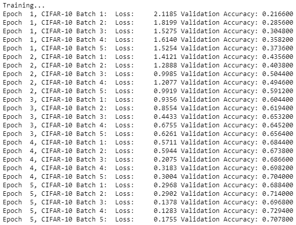
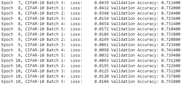
Now, the important part of Tensorflow Image Classification is done. Now, it’s time to test the model.
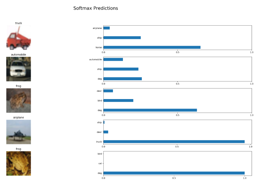
import pickle
import numpy as np
import matplotlib.pyplot as plt
from sklearn.preprocessing import LabelBinarizer

def batch_features_labels(features, labels, batch_size):
    """
    Split features and labels into batches
    """
    for start in range(0, len(features), batch_size):
        end = min(start + batch_size, len(features))
        yield features[start:end], labels[start:end]

def display_image_predictions(features, labels, predictions, top_n_predictions):
    n_classes = 10
    label_names = load_label_names()
    label_binarizer = LabelBinarizer()
    label_binarizer.fit(range(n_classes))
    label_ids = label_binarizer.inverse_transform(np.array(labels))

    fig, axies = plt.subplots(nrows=top_n_predictions, ncols=2, figsize=(20, 10))
    fig.tight_layout()
    fig.suptitle('Softmax Predictions', fontsize=20, y=1.1)

    n_predictions = 3
    margin = 0.05
    ind = np.arange(n_predictions)
    width = (1. - 2. * margin) / n_predictions

    for image_i, (feature, label_id, pred_indicies, pred_values) in enumerate(zip(features, label_ids, predictions.indices, predictions.values)):
        if (image_i < top_n_predictions):
            pred_names = [label_names[pred_i] for pred_i in pred_indicies]
            correct_name = label_names[label_id]

            axies[image_i][0].imshow((feature*255).astype(np.int32, copy=False))
            axies[image_i][0].set_title(correct_name)
            axies[image_i][0].set_axis_off()

            axies[image_i][1].barh(ind + margin, pred_values[:3], width)
            axies[image_i][1].set_yticks(ind + margin)
            axies[image_i][1].set_yticklabels(pred_names[::-1])
            axies[image_i][1].set_xticks([0, 0.5, 1.0])
%matplotlib inline
%config InlineBackend.figure_format = 'retina'

import tensorflow as tf
import pickle
import random

save_model_path = './image_classification'
batch_size = 64
n_samples = 10
top_n_predictions = 5

def test_model():
    test_features, test_labels = pickle.load(open('preprocess_training.p', mode='rb'))
    loaded_graph = tf.Graph()

    with tf.Session(graph=loaded_graph) as sess:
        # Load model
        loader = tf.train.import_meta_graph(save_model_path + '.meta')
        loader.restore(sess, save_model_path)

        # Get Tensors from loaded model
        loaded_x = loaded_graph.get_tensor_by_name('input_x:0')
        loaded_y = loaded_graph.get_tensor_by_name('output_y:0')
        loaded_keep_prob = loaded_graph.get_tensor_by_name('keep_prob:0')
        loaded_logits = loaded_graph.get_tensor_by_name('logits:0')
        loaded_acc = loaded_graph.get_tensor_by_name('accuracy:0')

        # Get accuracy in batches for memory limitations
        test_batch_acc_total = 0
        test_batch_count = 0

        for train_feature_batch, train_label_batch in batch_features_labels(test_features, test_labels, batch_size):
            test_batch_acc_total += sess.run(
                loaded_acc,
                feed_dict={loaded_x: train_feature_batch, loaded_y: train_label_batch, loaded_keep_prob: 1.0})
            test_batch_count += 1

        print('Testing Accuracy: {}
'.format(test_batch_acc_total/test_batch_count))

        # Print Random Samples
        random_test_features, random_test_labels = tuple(zip(*random.sample(list(zip(test_features, test_labels)), n_samples)))
        random_test_predictions = sess.run(
            tf.nn.top_k(tf.nn.softmax(loaded_logits), top_n_predictions),
            feed_dict={loaded_x: random_test_features, loaded_y: random_test_labels, loaded_keep_prob: 1.0})
        display_image_predictions(random_test_features, random_test_labels, random_test_predictions, top_n_predictions)


test_model()
Output: Testing Accuracy: 0.5882762738853503
Now, if you train your neural network for more epochs or change the activation function, you might get a different result that might have better accuracy.
Stay ahead of the curve in technology with This Post Graduate Program in AI and Machine Learning in partnership with E&ICT Academy, National Institute of Technology, Warangal. This Artificial Intelligence Course is curated to deliver the best results.
| Course Name | Date | Details |
|---|---|---|
| Artificial Intelligence Certification Course | Class Starts on 20th April,2024 20th April SAT&SUN (Weekend Batch) | View Details |
| Artificial Intelligence Certification Course | Class Starts on 8th June,2024 8th June SAT&SUN (Weekend Batch) | View Details |