
Data Science with Python Certification Course
- 132k Enrolled Learners
- Weekend
- Live Class
(49300)


 Copy Link!
_1648290501.jpg)
Statistics and Probability are the building blocks of the most revolutionary technologies in today’s world. From Artificial Intelligence to Machine Learning and Computer Vision, Statistics and Probability form the basic foundation to all such technologies. In this article on Statistics and Probability, I intend to help you understand the math behind the most complex algorithms and technologies.
To get in-depth knowledge on Data Science and the various Machine Learning Algorithms, you can enroll for live Data Science Certification Training by Edureka with 24/7 support and lifetime access.
The following topics are covered in this Statistics and Probability blog:
Look around you, there is data everywhere. Each click on your phone generates more data than you know. This generated data provides insights for analysis and helps us make better business decisions. This is why data is so important.
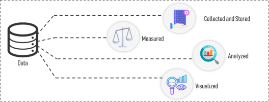
What Is Data – Statistics and Probability – Edureka
Data refers to facts and statistics collected together for reference or analysis.
Data can be collected, measured and analyzed. It can also be visualized by using statistical models and graphs.
Data can be categorized into two sub-categories:
Refer the below figure to understand the different categories of data:
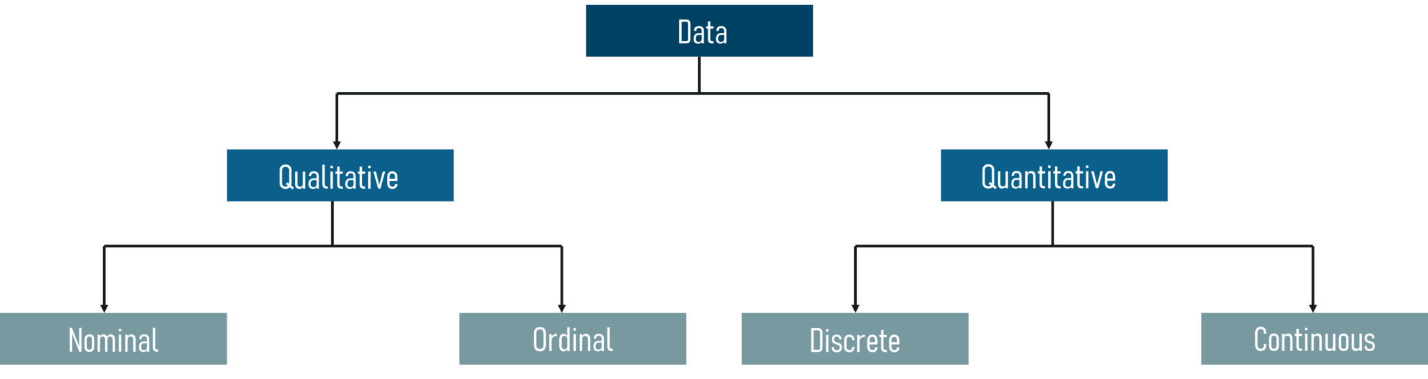
Categories Of Data – Statistics and Probability – Edureka
Qualitative Data: Qualitative data deals with characteristics and descriptors that can’t be easily measured, but can be observed subjectively. Qualitative data is further divided into two types of data:
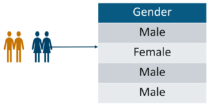
Nominal Data – Statistics and Probability – Edureka
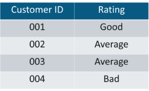
Ordinal Data – Statistics and Probability – Edureka
Quantitative Data: Quantitative data deals with numbers and things you can measure objectively. This is further divided into two:
Example: Number of students in a class.
So these were the different categories of data. The upcoming sections will focus on the basic Statistics concepts, so buckle up and get ready to do some math.
Statistics is an area of applied mathematics concerned with data collection, analysis, interpretation, and presentation.

What Is Statistics – Statistics and Probability – Edureka
This area of mathematics deals with understanding how data can be used to solve complex problems. Here are a couple of example problems that can be solved by using statistics:
These above-mentioned problems can be easily solved by using statistical techniques. In the upcoming sections, we will see how this can be done.
If you want a more in-depth explanation on Statistics and Probability, you can check out this video by our Statistics experts.
Before you dive deep into Statistics, it is important that you understand the basic terminologies used in Statistics. The two most important terminologies in statistics are population and sample.
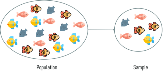
Population and Sample – Statistics and Probability – Edureka
Now you must be wondering how can one choose a sample that best represents the entire population.
Sampling is a statistical method that deals with the selection of individual observations within a population. It is performed to infer statistical knowledge about a population.
Consider a scenario wherein you’re asked to perform a survey about the eating habits of teenagers in the US. There are over 42 million teens in the US at present and this number is growing as you read this blog. Is it possible to survey each of these 42 million individuals about their health? Obviously not! That’s why sampling is used. It is a method wherein a sample of the population is studied in order to draw inference about the entire population.
There are two main types of Sampling techniques:
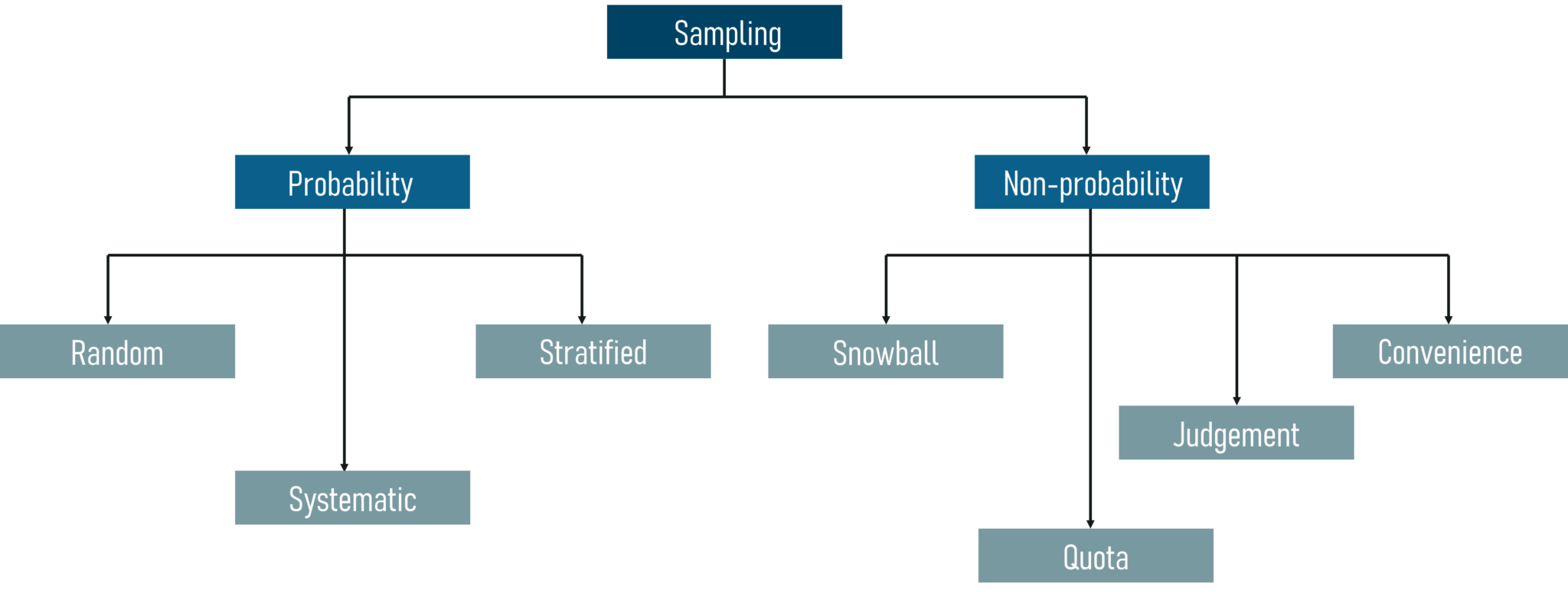
Sampling Techniques – Statistics and Probability – Edureka
In this blog, we’ll be focusing only on probability sampling techniques because non-probability sampling is not within the scope of this blog.
Probability Sampling: This is a sampling technique in which samples from a large population are chosen using the theory of probability. There are three types of probability sampling:

Random Sampling – Statistics and Probability – Edureka

Systematic Sampling – Statistics and Probability – Edureka
Stratified Sampling – Statistics and Probability – Edureka
Now that you know the basics of Statistics, let’s move ahead and discuss the different types of statistics.
There are two well-defined types of statistics:
Descriptive statistics is a method used to describe and understand the features of a specific data set by giving short summaries about the sample and measures of the data.
Descriptive Statistics is mainly focused upon the main characteristics of data. It provides a graphical summary of the data.

Descriptive Statistics – Statistics and Probability – Edureka
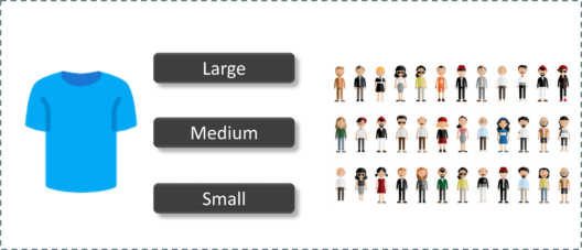
Suppose you want to gift all your classmate’s t-shirts. To study the average shirt size of students in a classroom, in descriptive statistics you would record the shirt size of all students in the class and then you would find out the maximum, minimum and average shirt size of the class.
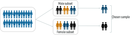
Inferential statistics makes inferences and predictions about a population based on a sample of data taken from the population in question.
Inferential statistics generalizes a large dataset and applies probability to draw a conclusion. It allows us to infer data parameters based on a statistical model using sample data.
Inferential Statistics – Statistics and Probability – Edureka
So, if we consider the same example of finding the average shirt size of students in a class, in Inferential Statistics, you will take a sample set of the class, which is basically a few people from the entire class. You already have had grouped the class into large, medium and small. In this method, you basically build a statistical model and expand it for the entire population in the class.
So that was a brief understanding of Descriptive and Inferential Statistics. In the further sections, you’ll see how Descriptive and Inferential statistics works in depth.
Descriptive Statistics is broken down into two categories:
Measures Of Centre
Measures of the center are statistical measures that represent the summary of a dataset. There are three main measures of center:
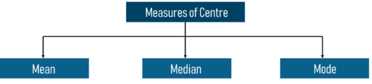
Measures Of Centre – Statistics and Probability – Edureka
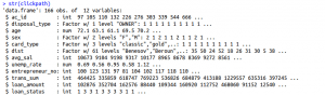
To better understand the Measures of central tendency let’s look at an example. The below cars dataset contains the following variables:
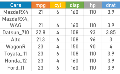
DataSet – Statistics and Probability – Edureka
Using descriptive Analysis, you can analyze each of the variables in the sample data set for mean, standard deviation, minimum and maximum.
If we want to find out the mean or average horsepower of the cars among the population of cars, we will check and calculate the average of all values. In this case, we’ll take the sum of the Horse Power of each car, divided by the total number of cars:
Mean = (110+110+93+96+90+110+110+110)/8 = 103.625
If we want to find out the center value of mpg among the population of cars, we will arrange the mpg values in ascending or descending order and choose the middle value. In this case, we have 8 values which is an even entry. Hence we must take the average of the two middle values.
The mpg for 8 cars: 21,21,21.3,22.8,23,23,23,23
Median = (22.8+23 )/2 = 22.9
If we want to find out the most common type of cylinder among the population of cars, we will check the value which is repeated the most number of times. Here we can see that the cylinders come in two values, 4 and 6. Take a look at the data set, you can see that the most recurring value is 6. Hence 6 is our Mode.
Measures Of The Spread
A measure of spread, sometimes also called a measure of dispersion, is used to describe the variability in a sample or population.
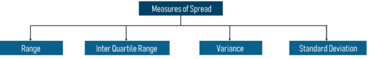
Measures Of Spread – Statistics and Probability – Edureka
Just like the measure of center, we also have measures of the spread, which comprises of the following measures:
Range = Max(𝑥_𝑖) – Min(𝑥_𝑖)
Here,
Max(𝑥_𝑖): Maximum value of x
Min(𝑥_𝑖): Minimum value of x
To better understand how quartile and the IQR are calculated, let’s look at an example.
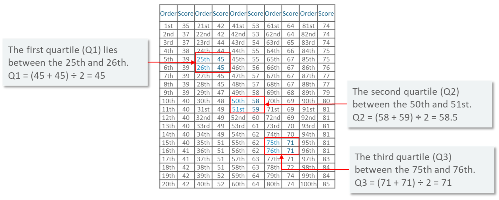
Measures Of Spread example – Statistics and Probability – Edureka
The above image shows marks of 100 students ordered from lowest to highest scores. The quartiles lie in the following ranges:
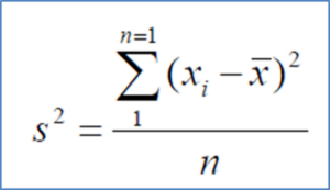
Measures Of Spread Variance – Statistics and Probability – Edureka
Here,
x: Individual data points
n: Total number of data points
x̅: Mean of data points
Deviation = (𝑥_𝑖 – µ)
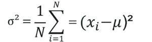
Measures Of Spread Population Variance – Statistics and Probability – Edureka
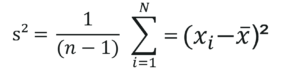
Measures Of Spread Sample Variance – Statistics and Probability – Edureka
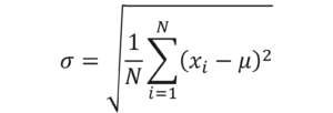
Measures Of Spread Standard Deviation – Statistics and Probability – Edureka
To better understand how the Measures of spread are calculated, let’s look at a use case.
Problem statement: Daenerys has 20 Dragons. They have the numbers 9, 2, 5, 4, 12, 7, 8, 11, 9, 3, 7, 4, 12, 5, 4, 10, 9, 6, 9, 4. Work out the Standard Deviation.
Let’s look at the solution step by step:
Step 1: Find out the mean for your sample set.
The mean is = 9+2+5+4+12+7+8+11+9+3
Then work out the mean of those squared differences.
+7+4+12+5+4+10+9+6+9+4 / 20
µ=7
Step 2: Then for each number, subtract the Mean and square the result.
(x_i – μ)²
(9-7)²= 2²=4
(2-7)²= (-5)²=25
(5-7)²= (-2)²=4
And so on…
We get the following results:
4, 25, 4, 9, 25, 0, 1, 16, 4, 16, 0, 9, 25, 4, 9, 9, 4, 1, 4, 9
Step 3: Then work out the mean of those squared differences.

4+25+4+9+25+0+1+16+4+16+0+9+25+4+9+9+4+1+4+9 / 20
⸫ σ² = 8.9
Step 4: Take the square root of σ².
σ = 2.983
To better understand the measures of spread and center, let’s execute a short demo by using the R language.
R is a statistical programming language, that is mainly used for Data Science, Machine Learning and so on. If you wish to learn more about R, give this R Tutorial – A Beginner’s Guide to Learn R Programming blog a read.
Now let’s move ahead and implement Descriptive Statistics in R.
In this demo, we’ll see how to calculate the Mean, Median, Mode, Variance, Standard Deviation and how to study the variables by plotting a histogram. This is quite a simple demo but it also forms the foundation that every Machine Learning algorithm is built upon.
Step 1: Import data for computation
set.seed(1)

#Generate random numbers and store it in a variable called data
>data = runif(20,1,10)
Step 2: Calculate Mean for the data
#Calculate Mean
>mean = mean(data)
>print(mean)

[1] 5.996504
Step 3: Calculate the Median for the data
#Calculate Median
>median = median(data)
>print(median)

[1] 6.408853
Step 4: Calculate Mode for the data
#Create a function for calculating Mode
>mode <- function(x) { >ux <- unique(x) >ux[which.max(tabulate(match(x, ux)))]}
>result <- mode(data) >print(data)

[1] 3.389578 4.349115 6.155680 9.173870 2.815137 9.085507 9.502077 6.947180 6.662026
[10] 1.556076 2.853771 2.589011 7.183206 4.456933 7.928573 5.479293 7.458567 9.927155
[19] 4.420317 7.997007

>cat("mode= {}", result)

mode= {} 3.389578
Step 5: Calculate Variance & Std Deviation for the data
#Calculate Variance and std Deviation
>variance = var(data)
>standardDeviation = sqrt(var(data))
>print(standardDeviation)

[1] 2.575061
Step 6: Plot a Histogram
#Plot Histogram
>hist(data, bins=10, range= c(0,10), edgecolor='black')
The Histogram is used to display the frequency of data points:

Histogram – Statistics And Probability – Edureka
Now that you know how to calculate the measure of the spread and center, let’s look at a few other statistical methods that can be used to infer the significance of a statistical model.
Entropy measures the impurity or uncertainty present in the data. It can be measured by using the below formula:

Entropy – Statistics and Probability – Edureka
where:
S – set of all instances in the dataset
N – number of distinct class values
pi – event probability
Information Gain (IG) indicates how much “information” a particular feature/ variable gives us about the final outcome. It can be measured by using the below formula:

Information Gain – Statistics and Probability – Edureka
Here:
Information Gain and Entropy are important statistical measures that let us understand the significance of a predictive model. To get a more clear understanding of Entropy and IG, let’s look at a use case.
Problem Statement: To predict whether a match can be played or not by studying the weather conditions.
Data Set Description: The following data set contains observations about the weather conditions over a period of time.
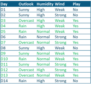
Use Case Dataset – Statistics and Probability – Edureka
The predictor variables include:
The target variable is the ‘Play’ variable which can be predicted by using the set of predictor variables. The value of this variable will decide whether or not a game can be played on a particular day.
To solve such a problem, we can make use of Decision Trees. Decision Trees are basically inverted trees that help us get to the outcome by making decisions at each branch node.
The below figure shows that out of 14 observations, 9 observations result in a ‘yes’, meaning that out of 14 days, the match can be played on 9 days. And if you notice, the decision was made by choosing the ‘Outlook’ variable as the root node (the topmost node in a Decision Tree).
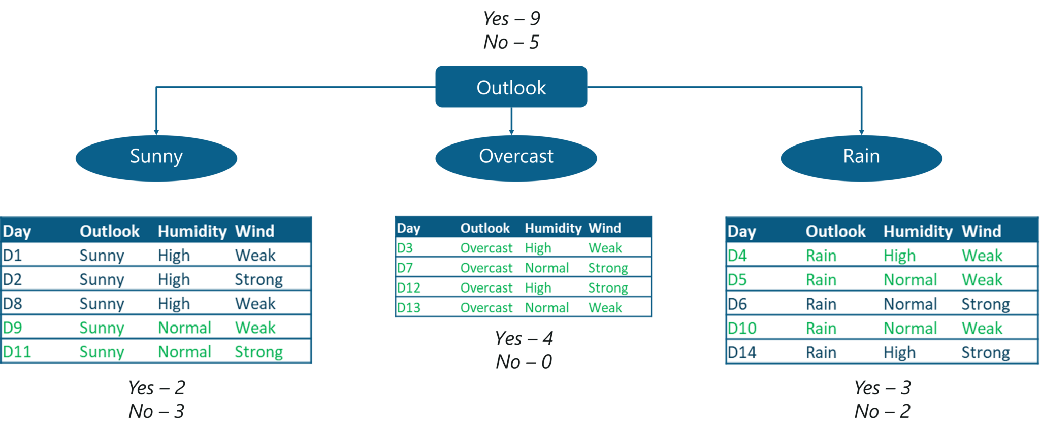
Use Case – Statistics and Probability – Edureka
The outlook variable has 3 values,
These 3 values are assigned to the immediate branch nodes and for each of these values, the possibility of ‘play= yes’ is calculated. The ‘sunny’ and ‘rain’ branches give out an impure output, meaning that there is a mix of ‘yes’ and ‘no’. But if you notice the ‘overcast’ variable, it results in a 100% pure subset. This shows that the ‘overcast’ variable will result in a definite and certain output.
This is exactly what entropy is used to measure. It calculates the impurity or the uncertainty and the lesser the uncertainty or the entropy of a variable, more significant is that variable.
In a Decision Tree, the root node is assigned the best attribute so that the Decision Tree can predict the most precise outcome. The ‘best attribute’ is basically a predictor variable that can best split the data set.
Now the next question in your head must be, “How do I decide which variable or attribute best splits the data?”
You can even check out the details of a successful Spark developers with the Pyspark training course.
Well, this can be done by using Information Gain and Entropy.
We begin by calculating the entropy when the ‘outlook’ variable is assigned to the root node. From the total of 14 instances we have:
The Entropy is:
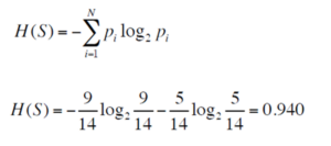
Calculating Entropy – Statistics and Probability – Edureka
Thus, we get an entropy of 0.940, which denotes impurity or uncertainty.
Now in order to ensure that we choose the best variable for the root node, let us look at all the possible combinations.
The below image shows each decision variable and the output that you can get by using that variable at the root node.
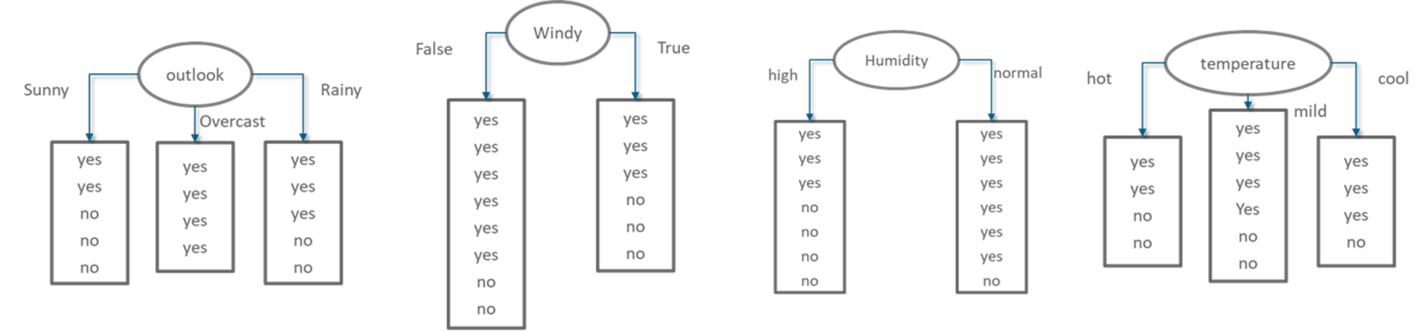
Possible Decision Trees- Statistics and Probability – Edureka
Our next step is to calculate the Information Gain for each of these decision variables (outlook, windy, humidity, temperature). A point to remember is, the variable that results in the highest IG must be chosen since it will give us the most precise output and information.
Information Gain of attribute “windy”
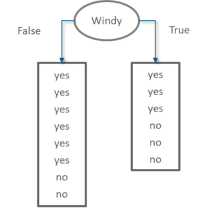
Decision Tree Windy – Statistics and Probability – Edureka
From the total of 14 instances we have:
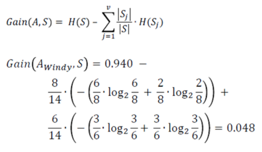
Information Gain windy – Statistics and Probability – Edureka
Information Gain of attribute “outlook”
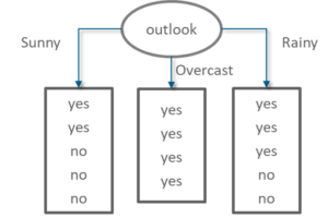
Decision Tree Outlook – Statistics and Probability – Edureka
From the total of 14 instances we have:
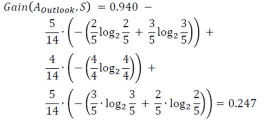
Information Gain outlook – Statistics and Probability – Edureka
Information Gain of attribute “humidity”
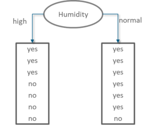
Decision Tree Humidity – Statistics and Probability – Edureka
From the total of 14 instances we have:
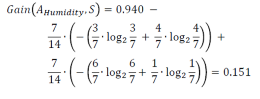
Information Gain humidity – Statistics and Probability – Edureka
Information Gain of attribute “temperature”
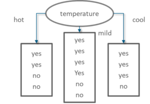
Decision Tree Temperature – Statistics and Probability – Edureka
From the total of 14 instances we have:
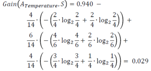
Information Gain temperature – Statistics and Probability – Edureka
The below figure shows the IG for each attribute. The variable with the highest IG is used to split the data at the root node. The ‘Outlook’ variable has the highest IG, therefore it is assigned to the root node.
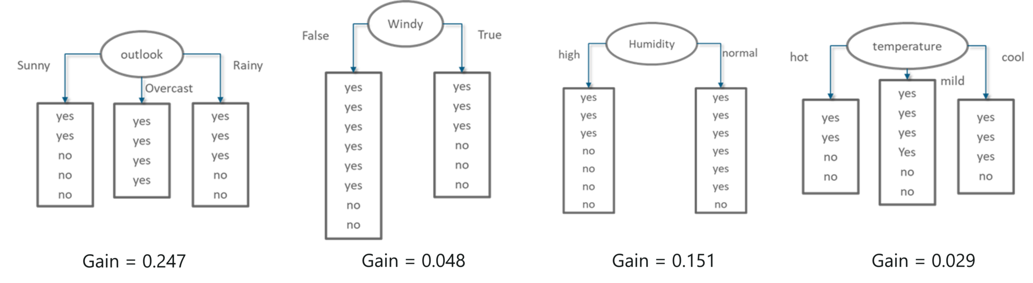
Information Gain Summary – Statistics and Probability – Edureka
So that was all about Entropy and Information Gain. Now let’s take a look at another important statistical method called Confusion Matrix.
A confusion matrix is a table that is often used to describe the performance of a classification model (or “classifier”) on a set of test data for which the true values are known.
Basically, a Confusion Matrix will help you evaluate the performance of a predictive model. It is mainly used in classification problems.
Confusion Matrix represents a tabular representation of Actual vs Predicted values. You can calculate the accuracy of a model by using the following formula:

Confusion Matrix Formula – Statistics and Probability – Edureka
To understand what is True Negative, True Positive and so on, let s consider an example.
Let’s consider that you’re given data about 165 patients, out of which 105 patients have a disease and the remaining 5o patients don’t. So you build a classifier that predicts by using these 165 observations. Out of those 165 cases, the classifier predicted “yes” 110 times, and “no” 55 times.
Therefore, in order to evaluate the efficiency of the classifier, a Confusion Matrix is used:
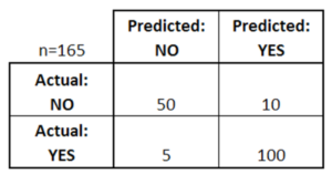
Confusion Matrix – Statistics and Probability – Edureka
In the above figure,
The confusion matrix studies the performance of the classifier by comparing the actual values to the predicted ones. Below are some terms related to the confusion matrix:
So those were the important concepts used in Descriptive Statistics. Now let’s study all about Probability.
Before we understand what probability is, let me clear out a very common misconception. People often tend to ask this question:
What is the relation between Statistics and Probability?
Probability and Statistics and related fields. Probability is a mathematical method used for statistical analysis. Therefore we can say that probability and statistics are interconnected branches of mathematics that deal with analyzing the relative frequency of events.
Now let’s understand what probability is.
Probability is the measure of how likely an event will occur. To be more precise probability is the ratio of desired outcomes to total outcomes:
(desired outcomes) / (total outcomes)
The probabilities of all outcomes always sums up to 1. Consider the famous rolling dice example:
Now let’s try to understand the common terminologies used in probability.
Before you dive deep into the concepts of probability, it is important that you understand the basic terminologies used in probability:
In this blog we shall focus on three main probability distribution functions:
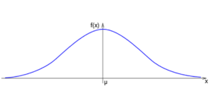
The Probability Density Function (PDF) is concerned with the relative likelihood for a continuous random variable to take on a given value. The PDF gives the probability of a variable that lies between the range ‘a’ and ‘b’.
The below graph denotes the PDF of a continuous variable over a range. This graph is famously known as the bell curve:
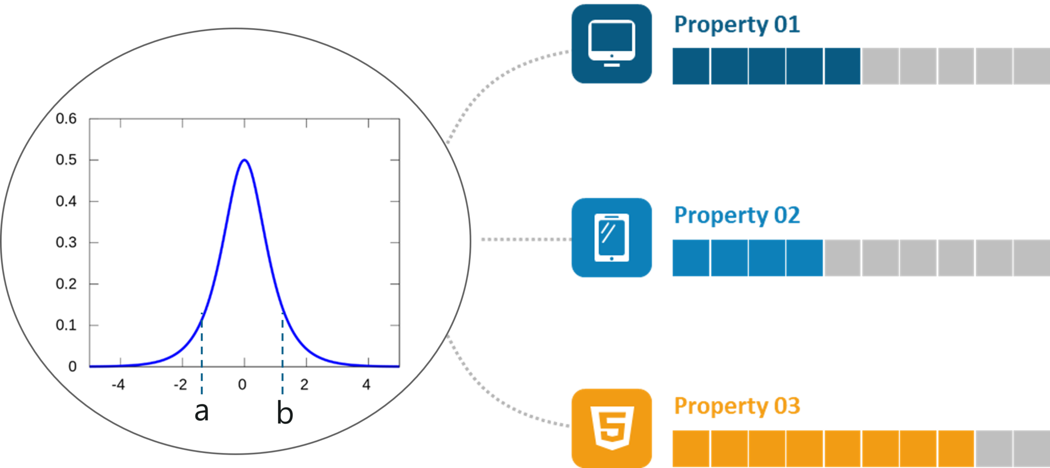
Probability Density Function – Statistics and Probability – Edureka
The following are the properties of a PDF:
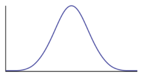
Normal distribution, otherwise known as the Gaussian distribution, is a probability distribution that denotes the symmetric property of the mean. The idea behind this function is that the data near the mean occurs more frequently than the data away from the mean. It infers that the data around the mean represents the entire data set.
Similar to PDF, the normal distribution appears as a bell curve:
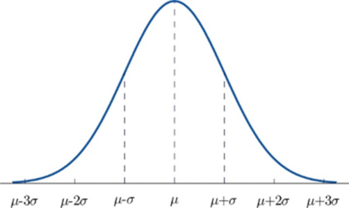
Normal Distribution – Statistics and Probability – Edureka
The graph of the Normal Distribution depends on two factors: the Mean and the Standard Deviation
If the standard deviation is large, the curve is short and wide:
Standard Deviation Curve – Statistics and Probability – Edureka
If the standard deviation is small, the curve is tall and narrow:
Standard Deviation Curve – Statistics and Probability – Edureka
The Central Limit Theorem states that the sampling distribution of the mean of any independent, random variable will be normal or nearly normal if the sample size is large enough.
In simple terms, if we had a large population divided into samples, then the mean of all the samples from the population will be almost equal to the mean of the entire population. The below graph depicts a more clear understanding of the Central Limit Theorem:
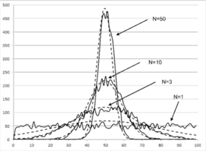
Central Limit Theorem – Statistics and Probability – Edureka
The accuracy or resemblance to the normal distribution depends on two main factors:
Now let’s focus on the three main types of probability.
The probability of an event occurring (p(A)), unconditioned on any other events. For example, the probability that a card drawn is a 3 (p(three)=1/13).
It can be expressed as:
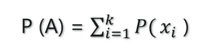
Marginal Probability – Statistics and Probability – Edureka
Joint Probability is a measure of two events happening at the same time, i.e., p(A and B), The probability of event A and event B occurring. It is the probability of the intersection of two or more events. The probability of the intersection of A and B may be written p(A ∩ B).
For example, the probability that a card is a four and red =p(four and red) = 2/52=1/26.
Probability of an event or outcome based on the occurrence of a previous event or outcome
Conditional Probability of an event B is the probability that the event will occur given that an event A has already occurred.
Example: Given that you drew a red card, what’s the probability that it’s a four (p(four|red))=2/26=1/13. So out of the 26 red cards (given a red card), there are two fours so 2/26=1/13.
Now let’s look at the last topic under probability.
The Bayes theorem is used to calculate the conditional probability, which is nothing but the probability of an event occurring based on prior knowledge of conditions that might be related to the event.
Mathematically, the Bayes theorem is represented as:
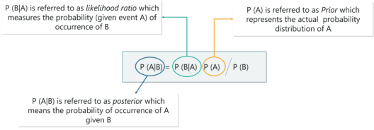
Bayes Theorem – Statistics and Probability – Edureka
In the above equation:
P(A|B): Conditional probability of event A occurring, given the event B
P(A): Probability of event A occurring
P(B): Probability of event B occurring
P(B|A): Conditional probability of event B occurring, given the event A
Formally, the terminologies of the Bayesian Theorem are as follows:
A is known as the proposition and B is the evidence
P(A) represents the prior probability of the proposition
P(B) represents the prior probability of evidence
P(A|B) is called the posterior
P(B|A) is the likelihood
Therefore, the Bayes theorem can be summed up as:
Posterior=(Likelihood).(Proposition prior probability)/Evidence prior probability
To better understand this, let’s look at an example:
Problem Statement: Consider 3 bags. Bag A contains 2 white balls and 4 red balls; Bag B contains 8 white balls and 4 red balls, Bag C contains 1 white ball and 3 red balls. We draw 1 ball from each bag. What is the probability to draw a white ball from Bag A if we know that we drew exactly a total of 2 white balls total?
Soln:

We can solve this problem in two steps:
Step 1: First find Pr(X). This can happen in three ways:
Step 2: Find Pr(A∩X).
I just drew out a blueprint to solve this problem. Consider this as homework and let us know your answer in the comment section.
The following section will cover the concepts under Inferential statistics, also known as Statistical Inference. So far we discussed Descriptive Statistics and Probability, now let’s look at a few more advanced topics.
As discussed earlier Statistical Inference is a branch of statistics that deals with forming inferences and predictions about a population based on a sample of data taken from the population in question.
The question you should ask now, is that how does one form inferences or predictions on a sample? The answer is through Point estimation.
Point Estimation is concerned with the use of the sample data to measure a single value which serves as an approximate value or the best estimate of an unknown population parameter.
Two important terminologies on Point Estimation are:
For example, in order to calculate the mean of a huge population, we first draw out a sample of the population and find the sample mean. The sample mean is then used to estimate the population mean. This is basically point estimation.
There are 4 common statistical techniques that are used to find the estimated value concerned with a population:
Apart from these four estimation methods, there is yet another estimation method known as Interval Estimation (Confidence Interval).
An Interval, or range of values, used to estimate a population parameter is known as Interval Estimation. The below image clearly shows what an Interval Estimation is as opposed to point estimation. The estimated value must occur between the lower confidence limit and the upper confidence limit.
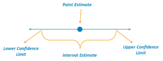
Interval Estimate – Statistics and Probability – Edureka
For example, if I stated that I will take 30 minutes to reach the theater, this is Point estimation. However, if I stated that I will take between 45 minutes to an hour to reach the theater, this is an example of Interval Estimation.
Interval Estimation gives rise to two important Statistical terminologies: Confidence Interval and Margin of Error.
For example, you survey a group of cat owners to see how many cans of cat food they purchase a year. You test your statistics at the 99 percent confidence level and get a confidence interval of (100,200). This means that you think they buy between 100 and 200 cans a year. And also since the Confidence Level is 99%, it shows that you’re very confident that the results are correct.
The Margin Of Error E can be calculated by using the below formula:

Margin Of Error – Statistics and Probability – Edureka
Here,
Now let’s understand how to estimate the Confidence Intervals.
The level of confidence ‘c’, is the probability that the interval estimate contains the population parameter. Consider the below figure:
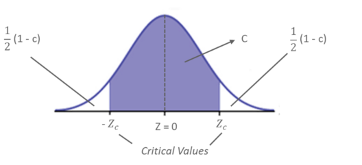
Estimating Level Of Confidence – Statistics and Probability – Edureka
For example, if the level of confidence is 90%, this means that you are 90% confident that the interval contains the population mean, 𝜇. The remaining 10% is equally distributed (0.05 ) on either side of ‘c’ (the area that contains the estimated population parameter)
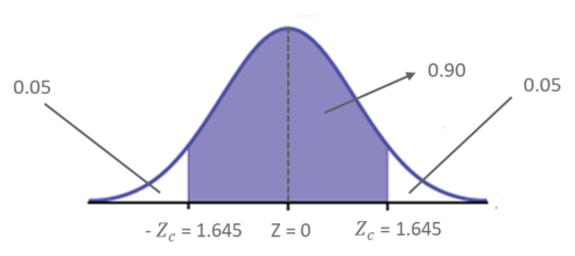
Estimating Level Of Confidence Example – Statistics and Probability – Edureka
The Corresponding Z – scores are ± 1.645 as per the Z table.
Construction Of Confidence Interval
The Confidence Interval can be constructed by following the below steps:
Now let’s look at a problem statement to better understand these concepts.
Problem Statement: A random sample of 32 textbook prices is taken from a local college bookstore. The mean of the sample is 𝑥 ̅ = 74.22, and the sample standard deviation is S = 23.44. Use a 95% confidence level and find the margin of error for the mean price of all textbooks in the bookstore
You know by formula, E = 𝑍_𝑐 * (𝜎/√𝑛)
E = 1.96 * (23.44/√32) ≈ 8.12
Therefore, we are 95% confident that the margin of error for the population mean (all the textbooks in the bookstore) is about 8.12.
Now that you know the idea behind Confidence Intervals, let’s move ahead to the next topic, Hypothesis Testing.
Statisticians use hypothesis testing to formally check whether the hypothesis is accepted or rejected. Hypothesis testing is an Inferential Statistical technique used to determine whether there is enough evidence in a data sample to infer that a certain condition holds true for an entire population.
To under the characteristics of a general population, we take a random sample and analyze the properties of the sample. We test whether or not the identified conclusion represents the population accurately and finally we interpret their results. Whether or not to accept the hypothesis depends upon the percentage value that we get from the hypothesis.
To better understand this, let’s look at an example.
Consider four boys, Nick, John, Bob and Harry who were caught bunking a class. They were asked to stay back at school and clean their classroom as a punishment.

Hypothesis Testing Example – Statistics and Probability – Edureka
So, John decided that the four of them would take turns to clean their classroom. He came up with a plan of writing each of their names on chits and putting them in a bowl. Every day they had to pick up a name from the bowl and that person must clean the class.
Now it has been three days and everybody’s name has come up, except John’s! Assuming that this event is completely random and free of bias, what is the probability of John not cheating?
Let’s begin by calculating the probability of John not being picked for a day:
P(John not picked for a day) = 3/4 = 75%
The probability here is 75%, which is fairly high. Now, if John is not picked for three days in a row, the probability drops down to 42%
P(John not picked for 3 days) = 3/4 ×3/4× 3/4 = 0.42 (approx)
Now, let’s consider a situation where John is not picked for 12 days in a row! The probability drops down to 3.2%. Thus, the probability of John cheating becomes fairly high.
P(John not picked for 12 days) = (3/4) ^12 = 0.032 <?.??
In order for statisticians to come to a conclusion, they define what is known as a threshold value. Considering the above situation, if the threshold value is set to 5%, it would indicate that, if the probability lies below 5%, then John is cheating his way out of detention. But if the probability is above the threshold value, then John is just lucky, and his name isn’t getting picked.
The probability and hypothesis testing give rise to two important concepts, namely:
Therefore, in our example, if the probability of an event occurring is less than 5%, then it is a biased event, hence it approves the alternate hypothesis.
To better understand Hypothesis Testing, we’ll be running a quick demo in the below section.
Hypothesis Testing In R
Here we’ll be using the gapminder data set to perform hypothesis testing. The gapminder data set contains a list of 142 countries, with their respective values for life expectancy, GDP per capita, and population, every five years, from 1952 to 2007.
The first step is to install and load the gapminder package into the R environment:
#Install and Load gapminder package
install.packages("gapminder")
library(gapminder)
data("gapminder")
Next, we’ll display the data set by using the View() function in R:
#Display gapminder dataset
View(gapminder)
Here’s a quick look at our data set:
 Data Set – Statistics And Probability – Edureka
The next step is to load the famous dplyr package provided by R.
#Install and Load dplyr package
install.packages("dplyr")
library(dplyr)
Our next step is to compare the life expectancy of two places (Ireland and South Africa) and perform the t-test to check if the comparison follows a Null Hypothesis or an Alternate Hypothesis.
#Comparing the variance in life expectancy in South Africa & Ireland
df1 <-gapminder %>%
select(country, lifeExp) %>%
filter(country == "South Africa" | country =="Ireland")
So, after you apply the t-test to the data frame (df1), and compare the life expectancy, you can see the below results:
#Perform t-test
t.test(data = df1, lifeExp ~ country)
Welch Two Sample t-test
data: lifeExp by country
t = 10.067, df = 19.109, p-value = 4.466e-09
alternative hypothesis: true difference in means is not equal to 0

95 percent confidence interval:
15.07022 22.97794
sample estimates:
mean in group Ireland mean in group South Africa
73.01725 53.99317
Notice the mean in group Ireland and in South Africa, you can see that life expectancy almost differs by a scale of 20. Now we need to check if this difference in the value of life expectancy in South Africa and Ireland is actually valid and not just by pure chance. For this reason, the t-test is carried out.
Pay special attention to the p-value also known as the probability value. The p-value is a very important measurement when it comes to ensuring the significance of a model. A model is said to be statistically significant only when the p-value is less than the pre-determined statistical significance level, which is ideally 0.05. As you can see from the output, the p-value is 4.466e-09 which is an extremely small value.
In the summary of the model, notice another important parameter called the t-value. A larger t-value suggests that the alternate hypothesis is true and that the difference in life expectancy is not equal to zero by pure luck. Hence in our case, the null hypothesis is disapproved.
So that was the practical implementation of Hypothesis Testing using the R language.
With this, we come to the end of this blog. If you have any queries regarding this topic, please leave a comment below and we’ll get back to you.
Stay tuned for more blogs on the trending technologies.
If you are looking for online structured training in Data Science, edureka! has a specially curated Data Science Course which helps you gain expertise in Statistics, Data Wrangling, Exploratory Data Analysis, Machine Learning Algorithms like K-Means Clustering, Decision Trees, Random Forest, Naive Bayes. You’ll learn the concepts of Time Series, Text Mining and an introduction to Deep Learning as well. New batches for this course are starting soon!!


 Thank you for registering Join Edureka Meetup community for 100+ Free Webinars each month JOIN MEETUP GROUP