SciPy Tutorial: What is Python SciPy and How to use it?

Mathematics deals with a huge number of concepts that are very important but at the same time, complex and time-consuming. However, Python provides the full-fledged SciPy library that resolves this issue for us. In this SciPy tutorial, you will be learning how to make use of this library along with a few functions and their examples.

Before moving on, take a look at all the topics discussed in this article:

• What is SciPy?
• NumPy vs SciPy
• Subpackages in SciPy
• Basic Functions
• Special Functions
• Integration Functions
• Optimization Functions
• Fourier Transform Functions
• Signal Processing Functions
• Linear Algebra
• Sparse Eigenvalues
• Spatial Data Structures and Algorithms
• Multidimensional Image Processing Functions
• File IO

So let’s get started. :)

What is SciPy?

SciPy is an open-source Python library which is used to solve scientific and mathematical problems. It is built on the NumPy extension and allows the user to manipulate and visualize data with a wide range of high-level commands. As mentioned earlier, SciPy builds on NumPy and therefore if you import SciPy, there is no need to import NumPy.

NumPy vs SciPy

Both NumPy and SciPy are Python libraries used for used mathematical and numerical analysis. NumPy contains array data and basic operations such as sorting, indexing, etc whereas, SciPy consists of all the numerical code. Though NumPy provides a number of functions that can help resolve linear algebra, Fourier transforms, etc, SciPy is the library that actually contains fully-featured versions of these functions along with many others. However, if you are doing scientific analysis using Python, you will need to install both NumPy and SciPy since SciPy builds on NumPy.

Subpackages in SciPy:

SciPy has a number of subpackages for various scientific computations which are shown in the following table:

However, for a detailed description, you can follow the official documentation.

These packages need to be imported exclusively prior to using them. For example:

from scipy import cluster

Before looking at each of these functions in detail, let’s first take a look at the functions that are common both in NumPy and SciPy.

Basic Functions:

Interaction with NumPy:

SciPy builds on NumPy and therefore you can make use of NumPy functions itself to handle arrays. To know in-depth about these functions, you can simply make use of help(), info() or source() functions.

help():

To get information about any function, you can make use of the help() function. There are two ways in which this function can be used:

• without any parameters
• using parameters

Here is an example that shows both of the above methods:

from scipy import cluster
help(cluster)               #with parameter
help()                       #without parameter

When you execute the above code, the first help() returns the information about the cluster submodule. The second help() asks the user to enter the name of any module, keyword, etc for which the user desires to seek information. To stop the execution of this function, simply type ‘quit’ and hit enter.

info():

This function returns information about the desired functions, modules, etc.

scipy.info(cluster) 

source():

The source code is returned only for objects written in Python. This function does not return useful information in case the methods or objects are written in any other language such as C. However in case you want to make use of this function, you can do it as follows:

scipy.source(cluster)

Special Functions:

SciPy provides a number of special functions that are used in mathematical physics such as elliptic, convenience functions, gamma, beta, etc. To look for all the functions, you can make use of help() function as described earlier.

Exponential and Trigonometric Functions:

SciPy’s Special Function package provides a number of functions through which you can find exponents and solve trigonometric problems.

Consider the following example:

EXAMPLE:

from scipy import special
a = special.exp10(3)
print(a)

b = special.exp2(3)
print(b)

c = special.sindg(90)
print(c)

d = special.cosdg(45)
print(d)

OUTPUT:

1000.0
8.0
1.0
0.7071067811865475

​There are many other functions present in the special functions package of SciPy that you can try for yourself.

Integration Functions:

SciPy provides a number of functions to solve integrals. Ranging from ordinary differential integrator to using trapezoidal rules to compute integrals, SciPy is a storehouse of functions to solve all types of integrals problems.

General Integration:

SiPy provides a function named quad to calculate the integral of a function which has one variable. The limits can be ±∞ (± inf) to indicate infinite limits. The syntax of the quad() function is as follows:

SYNTAX:

quad(func, a, b, args=(), full_output=0, epsabs=1.49e-08, epsrel=1.49e-08, limit=50, points=None, weight=None, wvar=None, wopts=None, maxp1=50, limlst=50)

Here, the function will be integrated between the limits a and b (can also be infinite).

EXAMPLE:

from scipy import special
from scipy import integrate
a= lambda x:special.exp10(x)
b = scipy.integrate.quad(a, 0, 1)
print(b)

In the above example, the function ‘a’ is evaluated between the limits 0, 1. When this code is executed, you will see the following output.

OUTPUT:

(3.9086503371292665, 4.3394735994897923e-14)

Double Integral Function:

SciPy provides dblquad that can be used to calculate double integrals. A double integral, as many of us know, consists of two real variables. The dblquad() function will take the function to be integrated as its parameter along with 4 other variables which define the limits and the functions dy and dx.

EXAMPLE:

from scipy import integrate
a = lambda y, x: x*y**2
b = lambda x: 1
c = lambda x: -1
integrate.dblquad(a, 0, 2, b, c)

OUTPUT:

-1.3333333333333335, 1.4802973661668755e-14)

SciPy provides various other functions to evaluate triple integrals, n integrals, Romberg Integrals, etc that you can explore further in detail. To find all the details about the required functions, use the help function.

Optimization Functions:

The scipy.optimize provides a number of commonly used optimization algorithms which can be seen using the help function.

It basically consists of the following:

• Unconstrained and constrained minimization of multivariate scalar functions i.e minimize (eg. BFGS, Newton Conjugate Gradient, Nelder_mead simplex, etc)
• Global optimization routines (eg. differential_evolution, dual_annealing, etc)
• Least-squares minimization and curve fitting (eg. least_squares, curve_fit, etc)
• Scalar univariate functions minimizers and root finders (eg. minimize_scalar and root_scalar)
• Multivariate equation system solvers using algorithms such as hybrid Powell, Levenberg-Marquardt.

Rosenbrook Function:

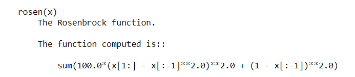
Rosenbrook function (rosen) is a test problem used for gradient-based optimization algorithms. It is defined as follows in SciPy:

EXAMPLE:

import numpy as np
from scipy.optimize import rosen
a = 1.2 * np.arange(5)
rosen(a)

OUTPUT: 7371.0399999999945

Nelder-Mead:

The Nelder–Mead method is a numerical method often used to find the min/ max of a function in a multidimensional space. In the following example, the minimize method is used along with the Nelder-Mead algorithm. 

EXAMPLE:

from scipy import optimize
a = [2.4, 1.7, 3.1, 2.9, 0.2]
b = optimize.minimize(optimize.rosen, a, method='Nelder-Mead')
b.x

OUTPUT:         array([0.96570182, 0.93255069, 0.86939478, 0.75497872, 0.56793357])

Interpolation Functions:

In the field of numerical analysis, interpolation refers to constructing new data points within a set of known data points. The SciPy library consists of a subpackage named scipy.interpolate that consists of spline functions and classes, one-dimensional and multi-dimensional (univariate and multivariate) interpolation classes, etc. 

Univariate Interpolation:

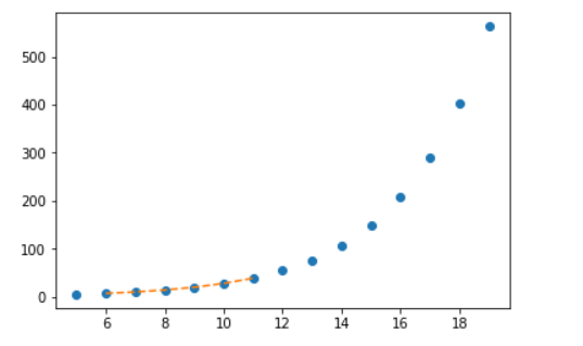
Univariate interpolation is basically an area of curve-fitting which finds the curve that provides an exact fit to a series of two-dimensional data points. SciPy provides interp1d function that can be utilized to produce univariate interpolation.

EXAMPLE:

import matplotlib.pyplot as plt
from scipy import interpolate
x = np.arange(5, 20)
y = np.exp(x/3.0)
f = interpolate.interp1d(x, y)x1 = np.arange(6, 12)
y1 = f(x1)   # use interpolation function returned by `interp1d`
plt.plot(x, y, 'o', x1, y1, '--')
plt.show()

OUTPUT:

Multivariate Interpolation:

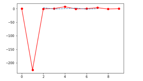
Multivariate interpolation (spatial interpolation ) is a kind interpolation on functions that consist of more than one variables. The following example demonstrates an example of the interp2d function.
Interpolating over a 2-D grid using the interp2d(x, y, z) function basically will use x, y, z arrays to approximate some function f: “z = f(x, y)“ and returns a function whose call method uses spline interpolation to find the value of new points.
EXAMPLE:

from scipy import interpolate
import matplotlib.pyplot as plt
x = np.arange(0,10)
y = np.arange(10,25)
x1, y1 = np.meshgrid(x, y)
z = np.tan(xx+yy)
f = interpolate.interp2d(x, y, z, kind='cubic')
x2 = np.arange(2,8)
y2 = np.arange(15,20)
z2 = f(xnew, ynew)
plt.plot(x, z[0, :], 'ro-', x2, z2[0, :], '--')
plt.show()

OUTPUT:

Fourier Transform Functions:

Fourier analysis is a method that deals with expressing a function as a sum of periodic components and recovering the signal from those components. The fft functions can be used to return the discrete Fourier transform of a real or complex sequence.

EXAMPLE:

from scipy.fftpack import fft, ifft
x = np.array([0,1,2,3])
y = fft(x)
print(y)

OUTPUT:   [ 6.+0.j -2.+2.j -2.+0.j -2.-2.j ]

Similarly, you can find the inverse of this by using the ifft function as follows:

EXAMPLE:

rom scipy.fftpack import fft, ifft
x = np.array([0,1,2,3])
y = ifft(x)
print(y)

OUTPUT:  [ 1.5+0.j -0.5-0.5j -0.5+0.j -0.5+0.5j]

Signal Processing Functions:

Signal processing deals with analyzing, modifying and synthesizing signals such as sound, images, etc. SciPy provides some functions using which you can design, filter and interpolate one-dimensional and two-dimensional data. 

Filtering:

By filtering a signal, you basically remove unwanted components from it. To perform ordered filtering, you can make use of the order_filter  function. This function basically performs ordered filtering on an array. The syntax of this function is as follows:

SYNTAX:
order_filter(a, domain, rank)

a = N-dimensional input array

domain = mask array having the same number of dimensions as `a`

rank = Non-negative number that selects elements from the list after it has been sorted (0 is the smallest followed by 1…)

EXAMPLE:

from scipy import signal
x = np.arange(35).reshape(7, 5)
domain = np.identity(3)
print(x,end='nn')
print(signal.order_filter(x, domain, 1))

OUTPUT:

[[ 0 1 2 3 4]
[ 5 6 7 8 9]
[10 11 12 13 14]
[15 16 17 18 19]
[20 21 22 23 24]
[25 26 27 28 29]
[30 31 32 33 34]]

[[ 0. 1. 2. 3. 0.]
[ 5. 6. 7. 8. 3.]
[10. 11. 12. 13. 8.]
[15. 16. 17. 18. 13.]
[20. 21. 22. 23. 18.]
[25. 26. 27. 28. 23.]
[ 0. 25. 26. 27. 28.]]

Waveforms:

The scipy.signal subpackage also consists of various functions that can be used to generate waveforms. One such function is chirp. This function is a frequency-swept cosine generator and the syntax is as follows:

SYNTAX:
chirp(t, f0, t1, f1, method=’linear’, phi=0, vertex_zero=True)

where,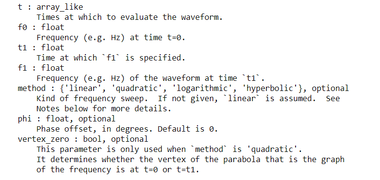

EXAMPLE:

from scipy.signal import chirp, spectrogram
import matplotlib.pyplot as plt
t = np.linspace(6, 10, 500)
w = chirp(t, f0=4, f1=2, t1=5, method='linear')
plt.plot(t, w)
plt.title("Linear Chirp")
plt.xlabel('time in sec)')
plt.show()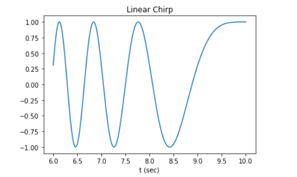

OUTPUT:

Linear Algebra:

Linear algebra deals with linear equations and their representations using vector spaces and matrices. SciPy is built on  ATLAS LAPACK and BLAS libraries and is extremely fast in solving problems related to linear algebra. In addition to all the functions from numpy.linalg, scipy.linalg also provides a number of other advanced functions. Also, if numpy.linalg is not used along with ATLAS LAPACK and BLAS support, scipy.linalg is faster than numpy.linalg. 

Finding the Inverse of a Matrix:

Mathematically, the inverse of a matrix A is the matrix B such that AB=I where I is the identity matrix consisting of ones down the main diagonal denoted as B=A^-1. In SciPy, this inverse can be obtained using the linalg.inv method. 

EXAMPLE:

import numpy as np
from scipy import linalg
A = np.array([[1,2], [4,3]])
B = linalg.inv(A)
print(B)

OUTPUT:

[[-0.6 0.4]
[ 0.8 -0.2]]

Finding the Determinants:

The value derived arithmetically from the coefficients of the matrix is known as the determinant of a square matrix. In SciPy, this can be done using a function det which has the following syntax:

SYNTAX:
det(a, overwrite_a=False, check_finite=True)
where,

a : (M, M) Is a square matrix

overwrite_a( bool, optional) : Allow overwriting data in a

check_finite ( bool, optional): To check whether input matrix consist only of finite numbers

EXAMPLE:

import numpy as np
from scipy import linalg
A = np.array([[1,2], [4,3]])
B = linalg.det(A)
print(B)

OUTPUT:  -5.0

Sparse Eigenvalues:

Eigenvalues are a specific set of scalars linked with linear equations. The ARPACK provides that allow you to find eigenvalues ( eigenvectors ) quite fast. The complete functionality of ARPACK is packed within two high-level interfaces which are scipy.sparse.linalg.eigs and scipy.sparse.linalg.eigsh. eigs. The eigs interface allows you to find the eigenvalues of real or complex nonsymmetric square matrices whereas the eigsh interface contains interfaces for real-symmetric or complex-hermitian matrices.

The eigh function solves a generalized eigenvalue problem for a complex Hermitian or real symmetric matrix.

EXAMPLE:

from scipy.linalg import eigh
import numpy as np
A = np.array([[1, 2, 3, 4], [4, 3, 2, 1], [1, 4, 6, 3], [2, 3, 2, 5]])
a, b = eigh(A)
print("Selected eigenvalues :", a)
print("Complex ndarray :", b)

OUTPUT:

Selected eigenvalues : [-2.53382695 1.66735639 3.69488657 12.17158399]
Complex ndarray : [[ 0.69205614 0.5829305 0.25682823 -0.33954321]
[-0.68277875 0.46838936 0.03700454 -0.5595134 ]
[ 0.23275694 -0.29164622 -0.72710245 -0.57627139]
[ 0.02637572 -0.59644441 0.63560361 -0.48945525]]

Spatial Data Structures and Algorithms:

Spatial data basically consists of objects that are made up of lines, points, surfaces, etc. The scipy.spatial package of SciPy can compute Voronoi diagrams, triangulations, etc using the Qhull library. It also consists of KDTree implementations for nearest-neighbor point queries. 

Delaunay triangulations:

Mathematically, Delaunay triangulations for a set of discrete points in a plane is a triangulation such that no point in the given set of points is inside the circumcircle of any triangle. 

EXAMPLE:

import matplotlib.pyplot as plt
from scipy.spatial import Delaunay
points = np.array([[0, 1], [1, 1], [1, 0],[0, 0]])
a = Delaunay(points)       #Delaunay object
print(a)
print(a.simplices)
plt.triplot(points[:,0], points[:,1], a.simplices)
plt.plot(points[:,1], points[:,0], 'o')
plt.show()

OUTPUT:

Multidimensional Image Processing Functions:

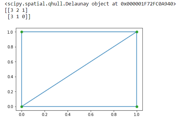
Image processing basically deals with performing operations on an image to retrieve information or to get an enhanced image from the original one. The scipy.ndimage package consists of a number of image processing and analysis functions designed to work with arrays of arbitrary dimensionality. 

Convolution and correlation:

SciPy provides a number of functions that allow correlation and convolution of images.

• The function correlate1d can be used to calculate one-dimensional correlation along a given axis
• The function correlate allows multidimensional correlation of any given array with the specified kernel
• The function convolve1d can be used to calculate one-dimensional convolution along a given axis
• The function convolve allows multidimensional convolution of any given array with the specified kernel

EXAMPLE:

import numpy as np
from scipy.ndimage import correlate1d
correlate1d([3,5,1,7,2,6,9,4], weights=[1,2])

OUTPUT:  array([ 9, 13, 7, 15, 11, 14, 24, 17])

File IO:

The scipy.io package provides a number of functions that help you manage files of different formats such as MATLAB files, IDL files, Matrix Market files, etc.

To make use of this package, you will need to import it as follows:

import scipy.io as sio

For complete information on subpackage, you can refer to the official document on File IO.

This brings us to the end of this SciPy Tutorial. I hope you have understood everything clearly. Make sure you practice as much as possible.

Got a question for us? Please mention it in the comments section of this “SciPy Tutorial” blog and we will get back to you as soon as possible.