
Data Science with Python Certification Course
- 132k Enrolled Learners
- Weekend
- Live Class
(49300)


 Copy Link!
With the demand for more complex computations, we cannot rely on simplistic algorithms. Instead, we must utilize algorithms with higher computational capabilities and one such algorithm is the Random Forest. In this blog post on Random Forest In R, you’ll learn the fundamentals of Random Forest along with its implementation by using the R Language.
To get in-depth knowledge on Data Science, you can enroll for live Data Science Certification Training by Edureka with 24/7 support and lifetime access.
Here’s a list of topics that I’ll be covering in this Random Forest In R blog:
Classification is the method of predicting the class of a given input data point. Classification problems are common in machine learning and they fall under the Supervised learning method.
Let’s say you want to classify your emails into 2 groups, spam and non-spam emails. For this kind of problems, where you have to assign an input data point into different classes, you can make use of classification algorithms.
Under classification we have 2 types:
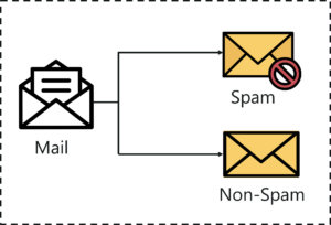
Classification – Random Forest In R – Edureka
The example that I gave earlier about classifying emails as spam and non-spam is of binary type because here we’re classifying emails into 2 classes (spam and non-spam).
But let’s say that we want to classify our emails into 3 classes:
So here we’re classifying emails into more than 2 classes, this is exactly what multi-class classification means.
One more thing to note here is that it is common for classification models to predict a continuous value. But this continuous value represents the probability of a given data point belonging to each output class.
Now that you have a good understanding of what classification is, let’s take a look at a few Classification Algorithms used in Machine Learning:
Random forest algorithm is a supervised classification and regression algorithm. As the name suggests, this algorithm randomly creates a forest with several trees.
Generally, the more trees in the forest the more robust the forest looks like. Similarly, in the random forest classifier, the higher the number of trees in the forest, greater is the accuracy of the results.
Random Forest – Random Forest In R – Edureka
In simple words, Random forest builds multiple decision trees (called the forest) and glues them together to get a more accurate and stable prediction. The forest it builds is a collection of Decision Trees, trained with the bagging method.
Before we discuss Random Forest in depth, we need to understand how Decision Trees work.
Many of you have this question in mind:
Let me explain.
Let’s say that you’re looking to buy a house, but you’re unable to decide which one to buy. So, you consult a few agents and they give you a list of parameters that you should consider before buying a house. The list includes:
These parameters are known as predictor variables, which are used to find the response variable. Here’s a diagrammatic illustration of how you can represent the above problem statement using a decision tree.
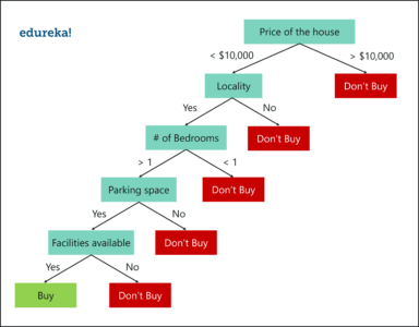
Decision Tree Example – Random Forest In R – Edureka
An important point to note here is that Decision trees are built on the entire data set, by making use of all the predictor variables.
Now let’s see how Random Forest would solve the same problem.
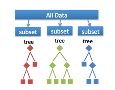
Like I mentioned earlier Random forest is an ensemble of decision trees, it randomly selects a set of parameters and creates a decision tree for each set of chosen parameters.
Take a look at the below figure.
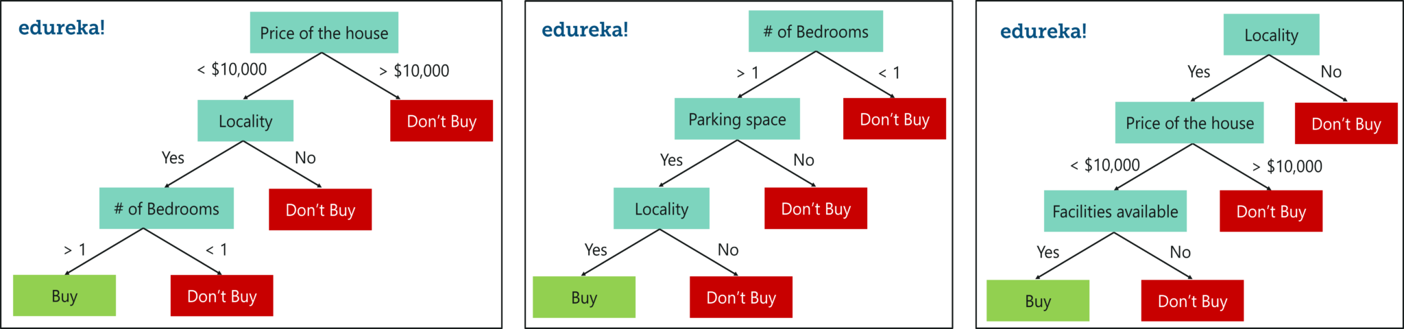
Random Forest With 3 Decision Trees – Random Forest In R – Edureka
Here, I’ve created 3 Decision Trees and each Decision Tree is taking only 3 parameters from the entire data set. Each decision tree predicts the outcome based on the respective predictor variables used in that tree and finally takes the average of the results from all the decision trees in the random forest.
In simple words, after creating multiple Decision trees using this method, each tree selects or votes the class (in this case the decision trees will choose whether or not a house is bought), and the class receiving the most votes by a simple majority is termed as the predicted class.
To conclude, Decision trees are built on the entire data set using all the predictor variables, whereas Random Forests are used to create multiple decision trees, such that each decision tree is built only on a part of the data set.
I hope the difference between Decision Trees and Random Forest is clear.
You might be wondering why we use Random Forest when we can solve the same problems using Decision trees. Let me explain.
This is where Random Forest comes in. It is based on the idea of bagging, which is used to reduce the variation in the predictions by combining the result of multiple Decision trees on different samples of the data set.
Now let’s focus on Random Forest.
To understand Random forest, consider the below sample data set. In this data set we have four predictor variables, namely:
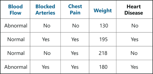
Sample Data Set – Random Forest In R – Edureka
These variables are used to predict whether or not a person has heart disease. We’re going to use this data set to create a Random Forest that predicts if a person has heart disease or not.
Step 1: Create a Bootstrapped Data Set
Bootstrapping is an estimation method used to make predictions on a data set by re-sampling it. To create a bootstrapped data set, we must randomly select samples from the original data set. A point to note here is that we can select the same sample more than once.
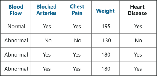
Bootstrapped Data Set – Random Forest In R – Edureka
In the above figure, I have randomly selected samples from the original data set and created a bootstrapped data set. Simple, isn’t it? Well, in real-world problems you’ll never get such a small data set, thus creating a bootstrapped data set is a little more complex.
Step 2: Creating Decision Trees
Just like this, we build the tree by only considering random subsets of variables at each step. By following the above process, our tree would look something like this:
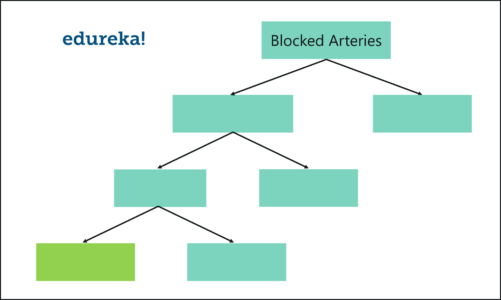
Random Forest Algorithm – Random Forest In R – Edureka
We just created our first Decision tree.
Step 3: Go back to Step 1 and Repeat
Like I mentioned earlier, Random Forest is a collection of Decision Trees. Each Decision Tree predicts the output class based on the respective predictor variables used in that tree. Finally, the outcome of all the Decision Trees in a Random Forest is recorded and the class with the majority votes is computed as the output class.
Thus, we must now create more decision trees by considering a subset of random predictor variables at each step. To do this, go back to step 1, create a new bootstrapped data set and then build a Decision Tree by considering only a subset of variables at each step. So, by following the above steps, our Random Forest would look something like this:
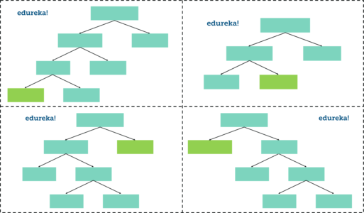
Random Forest – Random Forest In R – Edureka
This iteration is performed 100’s of times, therefore creating multiple decision trees with each tree computing the output, by using a subset of randomly selected variables at each step.
Having such a variety of Decision Trees in a Random Forest is what makes it more effective than an individual Decision Tree created using all the features and the whole data set.
Step 4: Predicting the outcome of a new data point
Now that we’ve created a random forest, let’s see how it can be used to predict whether a new patient has heart disease or not.
The below diagram has the data about the new patient. All we have to do is run this data down the decision trees that we made.
The first tree shows that the patient has heart disease, so we keep a track of that in a table as shown in the figure.
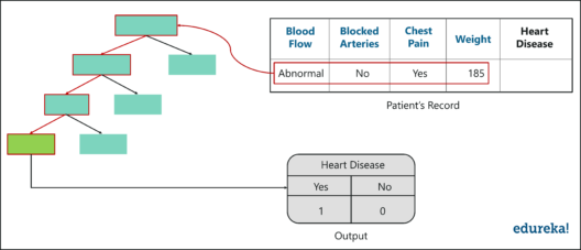
Output – Random Forest In R – Edureka
Similarly, we run this data down the other decision trees and keep a track of the class predicted by each tree. After running the data down all the trees in the Random Forest, we check which class got the majority votes. In our case, the class ‘Yes’ received the most number of votes, hence it’s clear that the new patient has heart disease.
To conclude, we bootstrapped the data and used the aggregate from all the trees to make a decision, this process is known as Bagging.
Step 5: Evaluate the Model
Our final step is to evaluate the Random Forest model. Earlier while we created the bootstrapped data set, we left out one entry/sample since we duplicated another sample. In a real-world problem, about 1/3rd of the original data set is not included in the bootstrapped data set.
The below figure shows the entry that didn’t end up in the bootstrapped data set.
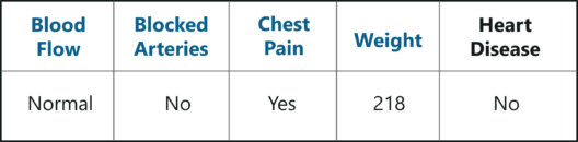
Out-Of-Bag Sample – Random Forest In R – Edureka
This sample data set that does not include in the bootstrapped data set is known as the Out-Of-Bag (OOB) data set.
In our case, the output class for the OOB data set is ‘No’. So, in order for our Random Forest model to be accurate, if we run the OOB data down the Decision trees, we must get a majority of ‘No’ votes. This process is carried out for all the OOB samples, in our case we only had one OOB, however, in most problems, there are usually many more samples.
Therefore, eventually, we can measure the accuracy of a Random Forest by the proportion of OOB samples that are correctly classified.
The proportion of OOB samples that are incorrectly classified is called the Out-Of-Bag Error. So that was an example of how Random Forest works.
Now let’s get our hands dirty and implement the Random Forest algorithm to solve a more complex problem.
Even people living under a rock would’ve heard of a movie called Titanic. But how many of you know that the movie is based on a real event? Kaggle assembled a data set containing data on who survived and who died on the Titanic.
Problem Statement: To build a Random Forest model that can study the characteristics of an individual who was on the Titanic and predict the likelihood that they would have survived.
Data Set Description: There are several variables/features in the data set for each person:
We’ll be running the below code snippets in R by using RStudio, so go ahead and open up RStudio. For this demo, you need to install the caret package and the randomForest package.
install.packages("caret", dependencies = TRUE)
install.packages("randomForest")
Next step is to load the packages into the working environment.
library(caret)
library(randomForest)
It’s time to load the data, we will use the read.table function to do this. Make sure you mention the path to the files (train.csv and test.csv)
train <- read.table('C:/Users/zulaikha/Desktop/titanic/train.csv', sep=",", header= TRUE)
The above command reads in the file “train.csv”, using the delimiter “,”, (which shows that the file is a CSV file) including the header row as the column names, and assigns it to the R object train.
Now, let’s read in the test data:
test <- read.table('C:/Users/zulaikha/Desktop/titanic/test.csv', sep = ",", header = TRUE)
To compare the training and testing data, let’s take a look at the first few rows of the training set:
head(train)
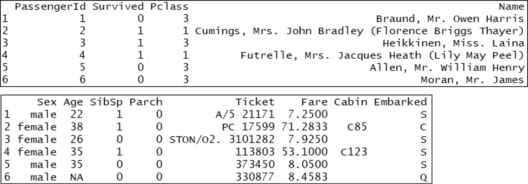
Training Data – Random Forest In R – Edureka
You’ll notice that each row has a column “Survived,” which is a probability between 0 and 1, if the person survived this value is above 0.5 and if they didn’t it is below 0.5. Now, let’s compare the training set to the test set:
head(test)
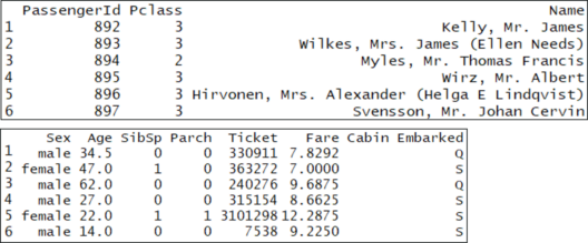
Testing Data – Random Forest In R – Edureka
The main difference between the training set and the test set is that the training set is labeled, but the test set is unlabeled. The train set obviously doesn’t have a column called “Survived” because we have to predict that for each person who boarded the titanic.
Before we get any further, the most essential factor while building a model is, picking the best features to use in the model. It’s never about picking the best algorithm or using the most sophisticated R package. Now, a “feature” is just a variable.
So, this brings us to the question, how do we pick the most significant variables to use? The easy way is to use cross-tabs and conditional box plots.
Cross-tabs represent relations between two variables in an understandable manner. In accordance to our problem, we want to know which variables are the best predictors for “Survived”. Let’s look at the cross-tabs between “Survived” and each other variable. In R, we use the table function:
table(train[,c('Survived', 'Pclass')])
        Pclass
Survived   1   2   3
       0  80  97 372
       1 136  87 119
From the cross-tab, we can see that “Pclass” could be a useful predictor of “Survived.” This is because, the first column of the cross-tab shows that, of the passengers in Class 1, 136 survived and 80 died (i.e. 63% of first-class passengers survived). On the other hand, in Class 2, 87 survived and 97 died (i.e. only 47% of second class passengers survived). Finally, in Class 3, 119 survived and 372 died (i.e. only 24% of third-class passengers survived). This means that there’s an obvious relationship between the passenger class and the survival chances.
Now we know that we must use Pclass in our model because it definitely has a strong predictive value of whether someone survived or not. Now, you can repeat this process for the other categorical variables in the data set, and decide which variables you want to include
To make things easier, let’s use the “conditional” box plots to compare the distribution of each continuous variable, conditioned on whether the passengers survived or not. But first we’ll need to install the ‘fields’ package:
install.packages("fields")
library(fields)
bplot.xy(train$Survived, train$Age)
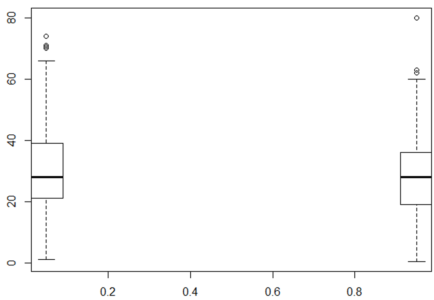
Box Plot – Random Forest In R – Edureka
The box plot of age for people who survived and who didn’t is nearly the same. This means that Age of a person did not have a large effect on whether one survived or not. The y-axis is Age and the x-axis is Survived.
Also, if you summarize it, there are lots of NA’s. So, let’s exclude the variable Age, because it doesn’t have a big impact on Survived, and because the NA’s make it hard to work with.
summary(train$Age)
   Min. 1st Qu.  Median    Mean 3rd Qu.    Max.    NA's
   0.42   20.12   28.00   29.70   38.00   80.00     177
In the below boxplot, the boxplot for Fares are much different for those who survived and those who didn’t. Again, the y-axis is Fare and the x-axis is Survived.
bplot.xy(train$Survived, train$Fare)
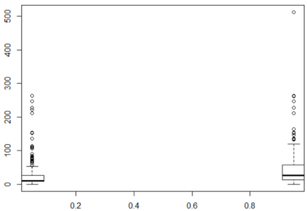
Box Plot For Fair – Random Forest In R – Edureka
On summarizing you’ll find that there are no NA’s for Fare. So, let’s include this variable.
summary(train$Fare)
   Min. 1st Qu.  Median    Mean 3rd Qu.    Max.
   0.00    7.91   14.45   32.20   31.00  512.33
The next step is to convert Survived to a Factor data type so that caret builds a classification instead of a regression model. After that, we use a simple train command to train the model.
Now the model is trained using the Random Forest algorithm that we discussed earlier. Random Forest is perfect for such problems because it performs numerous computations and predicts the results with high accuracy.
# Converting ‘Survived’ to a factor train$Survived <- factor(train$Survived) # Set a random seed set.seed(51) # Training using ‘random forest’ algorithm model <- train(Survived ~ Pclass + Sex + SibSp + Embarked + Parch + Fare, # Survived is a function of the variables we decided to include data = train, # Use the train data frame as the training data method = 'rf',# Use the 'random forest' algorithm trControl = trainControl(method = 'cv', # Use cross-validation number = 5) # Use 5 folds for cross-validation
To evaluate our model, we will use cross-validation scores.
Cross-validation is used to assess the efficiency of a model by using the training data. You start by randomly dividing the training data into 5 equally sized parts called “folds”. Next, you train the model on 4/5 of the data, and check its accuracy on the 1/5 of the data you left out. You then repeat this process with each split of the data. In the end, you average the percentage accuracy across the five different splits of the data to get an average accuracy. Caret does this for you, and you can see the scores by looking at the model output:
model
Random Forest

891 samples
  6 predictor
  2 classes: '0', '1'

No pre-processing
Resampling: Cross-Validated (5 fold)
Summary of sample sizes: 712, 713, 713, 712, 714
Resampling results across tuning parameters:

  mtry  Accuracy   Kappa
  2     0.8047116  0.5640887
  5     0.8070094  0.5818153
  8     0.8002236  0.5704306

Accuracy was used to select the optimal model using the largest value.
The final value used for the model was mtry = 5.
The first thing to notice is where it says, “The final value used for the model was mtry = 5.” The “mtry” is a hyper-parameter of the random forest model that determines how many variables the model uses to split the trees.
The table shows different values of mtry along with their corresponding average accuracy under cross-validation. Caret automatically picks the value of the hyper-parameter “mtry” that is the most accurate under cross-validation.
In the output, with mtry = 5, the average accuracy is 0.8170964, or about 82 percent. Which is the highest value, hence Caret picks this value for us.
Before we predict the output for the test data, let’s check if there is any missing data in the variables we are using to predict. If Caret finds any missing values, it will not return a prediction at all. So, we must find the missing data before moving ahead:
summary(test)
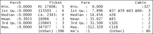
Summary of the Test Data – Random Forest In R – Edureka
Notice the variable “Fare” has one NA value. Let’s fill in that value with the mean of the “Fare” column. We use an if-else statement to do this.
So, if an entry in the column “Fare” is NA, then replace it with the mean of the column and remove the NA’s when you take the mean:
test$Fare <- ifelse(is.na(test$Fare), mean(test$Fare, na.rm = TRUE), test$Fare)
Now, our final step is to make predictions on the test set. To do this, you just have to call the predict method on the model object you trained. Let’s make the predictions on the test set and add them as a new column.
test$Survived <- predict(model, newdata = test)
Finally, it outputs the predictions for the test data,
test$Survived
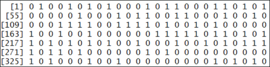
Predicting Outcome – Random Forest In R – Edureka
Here you can see the “Survived” values (either 0 or 1) for each passenger. Where one stands for survived and 0 stands for died. This prediction is made based on the “pclass” and “Fare” variables. You can use other variables too, if they are somehow related to whether a person boarding the titanic will survive or not.
Now that you know how Random Forest works, I’m sure you’re curious to learn more about the various Machine learning algorithms. Here’s a list of blogs that cover the different types of Machine Learning algorithms in depth
So, with this, we come to the end of this blog. I hope you all found this blog informative. If you have any thoughts to share, please comment them below. Stay tuned for more blogs like these!
If you are looking for online structured training in Data Science, edureka! has a specially curated Data Science course which helps you gain expertise in Statistics, Data Wrangling, Exploratory Data Analysis, Machine Learning Algorithms like K-Means Clustering, Decision Trees, Random Forest, Naive Bayes. You’ll learn the concepts of Time Series, Text Mining and an introduction to Deep Learning as well. New batches for this course are starting soon!!


 Thank you for registering Join Edureka Meetup community for 100+ Free Webinars each month JOIN MEETUP GROUP