R Shiny Tutorial: All you Need to Know

With the evolution of technology, newer tools and frameworks have emerged for building web-applications that display real-time statistics, maps, and graphs. Since these functionalities require high processing and synchronization, programming languages are used to reduce server-load time. In this R Shiny tutorial, I’ll explain how to make the best use of R on dynamic web applications.

We will cover and understand the following topics:

• • What is R Shiny?
  • Features of R Shiny
  • How is Shiny different from traditional applications?
  • Installing R Shiny
  • Structure of a Shiny app.
  • Create the first Shiny app.
  • Set up Shinyapps.io Account

What is R Shiny?

Shiny is an R package that allows users to build interactive web apps. This tool creates an HTML equivalent web app from Shiny code. We integrate native HTML and CSS code with R Shiny functions to make application presentable. Shiny combines the computational power of R with the interactivity of the modern web. Shiny creates web apps that are deployed on the web using your server or R Shiny’s hosting services.

Features of R Shiny:

• Create easy applications with basic or no knowledge of web tools
• Integrate Shiny with native web tools to improve flexibility and productivity
• Pre-built I/O and render functions
• Easy rendering of the application content without multiple reloads
• Feature to add computed (or processed) outputs from R scripts
• Add live reports and visualizations.

That brings us to the question:

How is Shiny different from traditional applications?

Lets us take an example of a weather application, whenever the user refreshes/loads the page or change any input, it should update the whole page or part of the page using JS. This adds load to the server-side for processing. Shiny allows the user to isolate or render(or reload) elements in the app which reduces server load. Scrolling through pages was easy in traditional web applications but was difficult with Shiny apps. The structure of the code plays the main role in understanding and debugging the code. This feature is crucial for shiny apps with respect to other applications.

Let’s move on to the next topic in R Shiny tutorial, installing the R Shiny package.

Installing R Shiny

Installing Shiny is like installing any other package in R. Go to R Console and run the below command to install the Shiny package.

install.packages("shiny")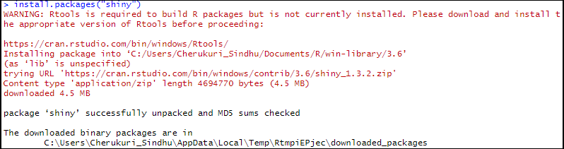

Once you have installed, load the Shiny package to create Shiny apps.

library(shiny)

Before we move any further in this R shiny tutorial, let’s see and understand the structure of a Shiny application.

Structure of a Shiny app

Shiny consists of 3 components:

1. User Interface
2. Server
3. ShinyApp

1. User Interface Function

User Interface (UI) function defines the layout and appearance of the app. You can add CSS and HTML tags within the app to make the app more presentable. The function contains all inputs and outputs to be displayed in the app. Each element (division or tab or menu) inside the app is defined using functions. These are accessed using a unique id, like HTML elements. Let’s learn further about various functions used in the app.

Shiny Layout Functions

• headerPanel()  add a heading to the app. titlePanel() defines subheading of the app. See the below image for a better understanding of headerPanel and titlePanel.
  

• SidebarLayout() defines layout to hold sidebarPanel and mainPanel elements. The layout divides app screen into sidebar panel and main panel. For example, in the below image, the red rectangle is the mainPanel area and the black rectangle area vertically is sidebarPanel area.

• wellPanel() defines a container that holds multiple objects app input/output objects in the same grid.
• tabsetPanel() creates a container to hold tabs. tabPanel() adds tab into the app by defining tab elements and components. In the below image, the black rectangle is tabsetPanel object and the red rectangle is the tabPanel object.
• navlistPanel() provides a side menu with links to different tab panels similar to tabsetPanel() like a Vertical list on the left side of the screen. In the below image, the black rectangle is navlistPanel object and the red rectangle is the tabPanel object.

Along with Shiny layout functions, you can also add inline CSS to each input widget in the app. The Shiny app incorporates features of the web technologies along with shiny R features and functions to enrich the app. Use HTML tags within the Shiny app using tags$<tag name>.

Your layout is ready, It’s time to add widgets into the app. Shiny provides various user input and output elements for user interaction. Let us discuss a few input and output functions.

Shiny Input Functions

Each input widget has a label, Id, other parameters such as choice, value, selected, min, max, etc.

• selectInput() – create a dropdown HTML element.

selectInput("select", h3("Select box"), choices = list("Choice 1" = 1,
 "Choice 2" = 2, "Choice 3" = 3), selected = 1)

• numericInput() – input area to type a number or text.

dateInput("num", "Date input", value = "2014-01-01")
numericInput("num", "Numeric input", value = 1)
textInput("num", "Numeric input", value = "Enter text...")

• radioButtons() – create radio buttons for user input.

radioButtons("radio", h3("Radio buttons"), choices = list("Choice 1" = 1,
"Choice 2" = 2,"Choice 3" = 3),selected = 1)

Shiny Output functions

Shiny provides various output functions that display R outputs such as plots, images, tables, etc which display corresponding R object.

• plotOutput() – display R plot object.

plotOutput"top_batsman")

•  tableOutput() – displays output as table.

tableOutput"player_table")

2. Server Function

Server function defines the server-side logic of the Shiny app. It involves creating functions and outputs that use inputs to produce various kinds of output.  Each client (web browser) calls the server function when it first loads the Shiny app. Each output stores the return value from the render functions.

These functions capture an R expression and do calculations and pre-processing on the expression. Use the render* function that corresponds to the output you are defining.  We access input widgets using input$[widget-id]. These input variables are reactive values. Any intermediate variables created using input variables need to be made reactive using reactive({ }). Access the variables using ( ).

render* functions perform the computation inside the server function and store in the output variables. The output needs to be saved with output$[output variable name]. Each render* function takes a single argument i.e, an R expression surrounded by braces, { }.

3. ShinyApp Function

shinyApp() function is the heart of the app which calls UI and server functions to create a Shiny App.

The below image shows the outline of the Shiny app.

Let’s move on to the next segment in the R Shiny tutorial to create the first R Shiny App.

Create a Shiny web project

Go to File and Create a New Project in any directory -> Shiny Web Application -> [Name of Shiny application Directory]. Enter the name of the directory and click OK.

Every new Shiny app project will contain a histogram example to understand the basics of a shiny app. The histogram app contains a slider followed by a histogram that updates the output for a change in the slider. Below is the output of the histogram app.

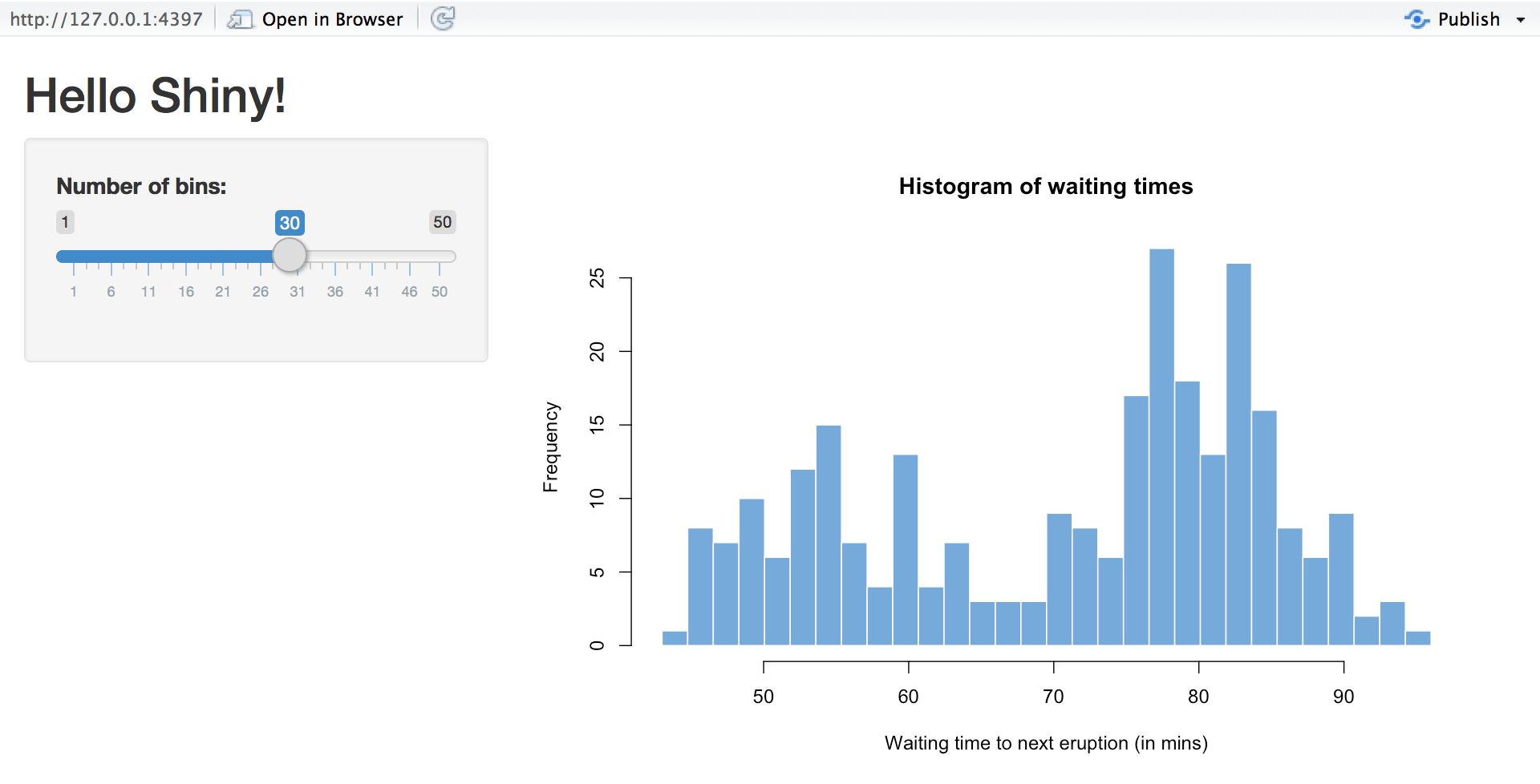
To run the Shiny app, click on the Run App button on the top right corner of the source pane. The Shiny app displays a slider widget which takes the number of bins as input and renders the histogram according to the input.

Now that you understood the structure and how to run a Shiny app. Let’s move on to create our first Shiny App.

Create the first Shiny app

You can either create a new project or continue in the same working directory. In this R Shiny tutorial, we will create a simple Shiny app to show IPL Statistics. The dataset used in the app can be downloaded here. The dataset comprises 2 files, deliveries.csv contains score deliveries for each ball (in over) batsman, bowler, runs details and matches.csv file contains match details such as match location, toss, venue & game details. The below app requires basic knowledge of dplyr and ggplot to understand the below tutorial.

Follow the below steps to create your first shiny app.

Step 1: Create the outline of a Shiny app.

Clear the existing code except for the function definitions in the app.R file.

Step 2: Load libraries and data.

In this step, we load the required packages and data. Then, clean and transform the extracted data into the required format. Add the below code before UI and server function.

Code:

library(shiny)
library(tidyverse)
# Loading Dataset-------------------------------------------------------
deliveries = read.csv("C:UsersCherukuri_SindhuDownloadsdeliveries.csv",
       stringsAsFactors = FALSE)
matches = read.csv("C:UsersCherukuri_SindhuDownloadsmatches.csv",
       stringsAsFactors = FALSE)
# Cleaning Dataset------------------------------------------------------
names(matches)[1] = "match_id"
IPL = dplyr::inner_join(matches,deliveries)

Explanation:

The first 2 lines load tidyverse and Shiny package. The next 2 lines load datasets deliveries and matches and store in variables deliveries and matches. The last 2 lines update the column name of the matches dataset to perform an inner join with the deliveries table. We store the join result in the IPL variable.

Step 3: Create the layout of Shiny app.

As discussed before, the UI function defines the app’s appearance, widgets, and objects in the Shiny app. Let’s discuss the same in detail.

Code

ui <- fluidPage(
   headerPanel("IPL - Indian Premier League"),
   tabsetPanel(
     tabPanel(title = "Season",
       mainPanel(width = 12,align = "center",
       selectInput("season_year","Select Season",choices=unique(sort(matches$season,
       decreasing=TRUE)), selected = 2019),
       submitButton("Go"),
       tags$h3("Players table"),
       div(style = "border:1px black solid;width:50%",tableOutput("player_table"))
)),
     tabPanel(
       title = "Team Wins & Points",
       mainPanel(width = 12,align = "center",
       tags$h3("Team Wins & Points"),
       div(style = "float:left;width:36%;",plotOutput("wins_bar_plot")),
       div(style = "float:right;width:64%;",plotOutput("points_bar_plot"))
)
)))

The UI function contains a headerPanel() or titlePanel() and followed by tabsetPanel to define multiple tabs in the app. tabPanel() defines the objects for each tab, respectively. Each tabPanel() consists of title and mainPanel(). mainPanel() creates a container of width 12 i.e full window and align input and output objects in the center.

Explanation

The app consists of 2 tabs: Season and Team Wins & Points.

Season tab consists of selectInput(), submit button and a table. season_year is used to read input from the list of values. tableOutput() displays table output calculated on server function. Table player_table is displayed below button which is defined in server function which shall be discussed in the next step. Team Wins & Points tab displays team-wise win and points in respective bar charts. plotOutput() displays outputs returned from render* functions. All the output, input functions are enclosed within a div tag to add inline styling.

Now that we are familiar with ui function, let’s go ahead with understanding and using server function in our R Shiny tutorial.

Step 4: Add the server function statements

The server function involves creating functions and outputs that use user inputs to produce various kinds of output. The server function is explained step by step below. 

matches_year = reactive({ matches %>% filter(season == input$season_year) })
playoff = reactive({ nth(sort(matches_year()$match_id,decreasing = TRUE),4) })
matches_played = reactive({ matches_year()&nbsp;%>% filter(match_id < playoff()) }) t1 = reactive({ matches_played()&nbsp;%>% group_by(team1)&nbsp;%>% summarise(count = n()) })
t2 = reactive({ matches_played()&nbsp;%>% group_by(team2)&nbsp;%>% summarise(count = n()) })
wl = reactive({ matches_played()&nbsp;%>% filter(winner&nbsp;!= "")&nbsp;%>% group_by(winner)&nbsp;%>% 
summarise(no_of_wins = n()) })
    
wl1=reactive({ matches_played()&nbsp;%>% group_by(winner)&nbsp;%>% summarise(no_of_wins=n()) })
tied = reactive({ matches_played()&nbsp;%>% filter(winner == "")&nbsp;%>% select(team1,team2) })
playertable = reactive({data.frame(Teams = t1()$team1,Played=t1()$count+t2()$count,
Wins = wl()$no_of_wins,Points = wl()$no_of_wins*2)})

The above code filter matches played before playoffs each year, and store the result in the matches_played variable. player_table table contains team-wise match statistics i.e played, wins, and points. Variables matches_played, player_table, t1, tied, etc are all intermediate reactive values. These variables need to be accessed using ( ) as shown in the code above. player_table is displayed using renderTable function. Next, create the output variable to store playertable.

output$player_table = renderTable({ playertable() })

Now lets create bar charts to show wins and points scored by each team in the season. The below code displays bar charts using ggplot. renderPlot() fetches ggplot object and store the result in variable wins_bar_plot.The ggplot code is self-explanatory, it involves basic graphics and mapping functions to edit legend, labels and plot.

output$wins_bar_plot = renderPlot({ ggplot(wl1()[2:9,],aes(winner,no_of_wins,fill=winner))+
geom_bar(stat = "identity")+ theme_classic()+xlab("Teams")+ ylab("Number Of Wins")+theme(
axis.text.x=element_text(color="white"),legend.position = "none",axis.title=element_text(
size=14),plot.background=element_rect(colour="white"))+geom_text(aes(x=winner,(no_of_wins+0.6),
label = no_of_wins,size = 7)) })

output$points_bar_plot = renderPlot({ ggplot(playertable(),aes(Teams,Points,fill=Teams))+
geom_bar(stat = "identity",size=3)+theme_classic()+theme(axis.text.x=element_text(
color = "white"),legend.text = element_text(size = 14),axis.title = element_text(size=14))+
geom_text(aes(Teams,(Points+1),label=Points,size = 7)) })

Step 5: Run the Shiny app.

Click on Run App. With a successful run, your Shiny app will look like below. Any error or warnings related to the app, it will display these in R Console.

Tab1 – Season

Tab2 – Team Wins & Points

Let’s see how to set up Shinyapps.io account to deploy your Shiny apps.

Set up Shinyapps.io Account

Go to Shinyapps.io and sign in with your information, then give a unique account name for the page and save it. After saving successfully, you will see a detailed procedure to deploy apps from the R Console. Follow the below procedure to configure your account in Rstudio.

Step 1. Install rsconnect

install.packages('rsconnect')

Step 2. Authorize Account

The rsconnect package must be authorized to your account using a token and secret. To do this, copy the whole command as shown below in your dashboard page in R console. Once you’ve entered the command successfully in R, I now authorize you to deploy applications to your Shinyapps.io account.

rsconnect::setAccountInfo(name='account name',token='token',
              secret="secret")

Step 3. Deploy App

Use the below code to deploy Shiny apps.

library(rsconnect)
rsconnect::deployApp('path/to/your/app')

Once set, you are ready to deploy your shiny apps.

Now that you learned how to create and run Shiny apps, deploy the app we just created into Shinyapps.io as explained above or click on publish, which is present on the top right corner of the Shiny app window.

I hope that this R Shiny tutorial helped you learn how to create and run a Shiny app. Have fun creating interactive and beautiful web apps using R Shiny.

If you wish to learn R Programming and build a colorful career in Data Analytics, then check out our Data Analytics using R which comes with instructor-led live training and real-life project experience. This training will help you understand data analytics and help you achieve mastery over the subject.