Q Learning: All you need to know about Reinforcement Learning

Artificial Intelligence and Machine Learning are a few domains that are amongst the top buzzwords in the industry and for a good reason. AI is going to create 2.3 million jobs by 2020 considering its main goal is to enable machines to mimic human behavior. Odd isn’t it? So, today we are going to discuss Q Learning, the building block of Reinforcement Learning in the following order:

• What is Reinforcement Learning?
• Q-Learning Process
• Bellman Equation
• Markov Decision Process
• Q-Learning Demo: NumPy

What is Reinforcement Learning?

Let’s have a look at our day to day life. We perform numerous tasks in the environment and some of those tasks bring us rewards while some do not. We keep looking for different paths and try to find out which path will lead to rewards and based on our action we improve our strategies on achieving goals. This my friends are one of the simplest analogy of Reinforcement Learning.

Key areas of Interest :

• Environment
• Action
• Reward
• State

Reinforcement Learning is the branch of machine learning that permits systems to learn from the outcomes of their own decisions. It solves a particular kind of problem where decision making is sequential, and the goal is long-term.

Check out this NLP Training by Edureka to upgrade your AI skills to the next level

Q-Learning Process

Let’s understand what is Q learning with our problem statement here. It will help us to define the main components of a reinforcement learning solution i.e. agents, environment, actions, rewards, and states.

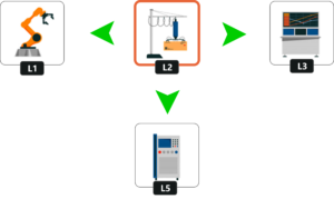
Automobile Factory Analogy:

We are at an Automobile Factory filled with robots. These robots help the Factory workers by conveying the necessary parts required to assemble a car. These different parts are located at different locations within the factory in 9 stations. The parts include Chassis, Wheels, Dashboard, Engine and so on. Factory Master has prioritized the location where chassis is being installed as the highest priority. Let’s have a look at the setup here:

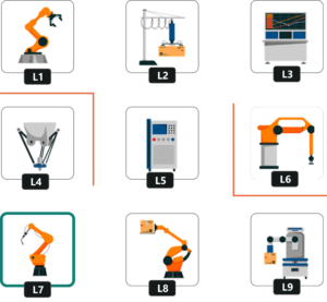
States:

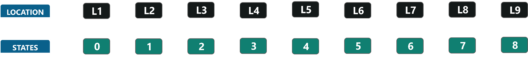
The Location at which a robot is present at a particular instance is called its state. Since it is easy to code it rather than remembering it by names. Let’s map the location to numbers.

Actions:

Actions are nothing but the moves made by the robots to any location. Consider, a robot is at the L2 location and the direct locations to which it can move are L5, L1 and L3. Let’s understand this better if we visualize this:

Rewards:

A Reward will be given to the robot for going directly from one state to another. For example, you can reach L5 directly from L2 and vice versa. So, a reward of 1 will be provided in either case. Let’s have a look at the reward table:

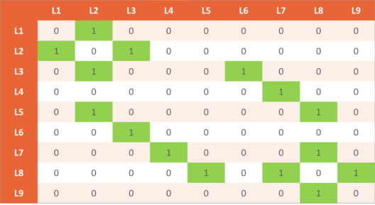
Remember when the Factory Master Prioritized the chassis location. It was L7, so we are going to incorporate this fact into our rewards table. So, we’ll assign a very large number(999 in our case) in the (L7, L7) location.

Bellman Equation

Now suppose a robot needs to go from point A to B. It will choose the path which will yield a positive reward. For that suppose we provide a reward in terms of footprint for it to follow.

But what if the robot starts from somewhere in between where it can see two or more paths. The robot can thus not take a decision and this primarily happens because it doesn’t possess a memory. This is where the Bellman Equation comes into the picture.

V(s) = max(R(s,a) + 𝜸V(s’))

Where:

• s = a particular state
• a = action
• s′ = state to which the robot goes from s
• 𝜸 = discount factor
• R(s, a) = a reward function which takes a state (s) and action (a) and outputs a reward value
• V(s) = value of being in a particular state

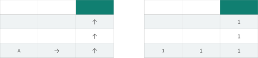
Now the block below the destination will have a reward of 1, which is the highest reward, But what about the other block? Well, this is where the discount factor comes in. Let’s assume a discount factor of 0.9 and fill all the blocks one by one.

Markov Decision Process

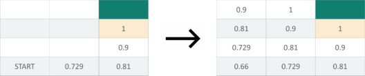
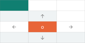
Imagine a robot is on the orange block and needs to reach the destination. But even if there is a slight dysfunction the robot will be confused about which path to take rather than going up.

So we need to modify the decision-making process. It has to Partly Random and Partly under the robot’s control. Partly Random because we don’t know when the robot will dysfunction and Partly under control because it’s still the robot’s decision. And this forms the base for the Markov Decision Process.

A Markov decision process (MDP) is a discrete time stochastic control process. It provides a mathematical framework for modeling decision making in situations where outcomes are partly random and partly under the control of a decision maker.

So we are going to use our original Bellman equation and make changes in it. What we don’t know is the next state ie. s’. What we know is all the possibilities of a turn and let’s change the Equation.

V(s) = max(R(s, a) + 𝜸 V(s’))

V(s) = max(R(s, a) + 𝜸 Σ _s’ P(s, a, s’) V(s’))

P(s,a,s’) : Probability of moving from state s to s’ with action a

Σ _s’ P(s,a,s’) V(s’) : Randomness Expectations of Robot

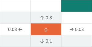
V(s) = max(R(s, a) + 𝜸 ((0.8V(room _up)) + (0.1V(room _down) + ….))

Now, Let’s transition into Q Learning. Q-Learning poses an idea of assessing the quality of an action that is taken to move to a state rather than determining the possible value of the state it is being moved to.

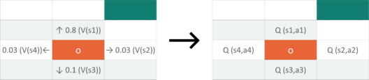
This is what we get if we incorporate the idea of assessing the quality of actions for moving to a certain state s′.  From the updated Bellman Equation if we remove them max component, we are assuming only one footprint for possible action which is nothing but the Quality of the action.

Q(s, a) = (R(s, a) + 𝜸 Σ _s’ P(s, a, s’) V(s’))

In this equation that Quantifies the Quality of action, we can assume that V(s) is the maximum of all possible values of Q(s, a). So let’s replace v(s’) with a function of Q().

Q(s, a) = (R(s, a) + 𝜸 Σ _s’ P(s, a, s’) max Q(s’, a’))

We are just one step close to our final Equation of Q Learning. We are going to introduce a Temporal Difference to calculate the Q-values with respect to the changes in the environment over time. But how do we observe the change in Q?

TD(s, a) = (R(s, a) + 𝜸 Σ _s’ P(s, a, s’) max Q(s’, a’)) – Q(s, a)

We recalculate the new Q(s, a) with the same formula and subtract the previously known Q(s, a) from it. So, the above equation becomes:

Q_t (s, a) = Q_t-1 (s, a) + α TD_t (s, a)

Q_t (s, a) = Current Q-value

Q_t-1 (s, a) = Previous Q-value

Q_t (s, a) = Q_t-1 (s, a) + α (R(s, a) + 𝜸 max Q(s’, a’) _– Q_t-1(s, a))

Q Learning Demo: NumPy

I am going to use Python NumPy to demonstrate how Q Learning works.

Step 1: Imports, Parameters, States, Actions, and Rewards

import numpy as np

gamma = 0.75 # Discount factor
alpha = 0.9 # Learning rate

location_to_state = {
    'L1' : 0,
    'L2' : 1,
    'L3' : 2,
    'L4' : 3,
    'L5' : 4,
    'L6' : 5,
    'L7' : 6,
    'L8' : 7,
    'L9' : 8
}

actions = [0,1,2,3,4,5,6,7,8]

rewards = np.array([[0,1,0,0,0,0,0,0,0],
              [1,0,1,0,0,0,0,0,0],
              [0,1,0,0,0,1,0,0,0],
              [0,0,0,0,0,0,1,0,0],
              [0,1,0,0,0,0,0,1,0],
              [0,0,1,0,0,0,0,0,0],
              [0,0,0,1,0,0,0,1,0],
              [0,0,0,0,1,0,1,0,1],
              [0,0,0,0,0,0,0,1,0]])

Step 2:  Map Indices to locations

state_to_location = dict((state,location) for location,state in location_to_state.items())

Step 3: Get Optimal Route using Q Learning Process

def get_optimal_route(start_location,end_location):
    rewards_new = np.copy(rewards)
    ending_state = location_to_state[end_location]
    rewards_new[ending_state,ending_state] = 999

    Q = np.array(np.zeros([9,9]))

    # Q-Learning process
    for i in range(1000):
        # Picking up a random state
        current_state = np.random.randint(0,9) # Python excludes the upper bound
        playable_actions = []
        # Iterating through the new rewards matrix
        for j in range(9):
            if rewards_new[current_state,j] > 0:
                playable_actions.append(j)
        # Pick a random action that will lead us to next state
        next_state = np.random.choice(playable_actions)
        # Computing Temporal Difference
        TD = rewards_new[current_state,next_state] + gamma * Q[next_state, np.argmax(Q[next_state,])] - Q[current_state,next_state]
        # Updating the Q-Value using the Bellman equation
        Q[current_state,next_state] += alpha * TD

    # Initialize the optimal route with the starting location
    route = [start_location]
    #Initialize next_location with starting location
    next_location = start_location

    # We don't know about the exact number of iterations needed to reach to the final location hence while loop will be a good choice for iteratiing
    while(next_location != end_location):
        # Fetch the starting state
        starting_state = location_to_state[start_location]
        # Fetch the highest Q-value pertaining to starting state
        next_state = np.argmax(Q[starting_state,])
        # We got the index of the next state. But we need the corresponding letter.
        next_location = state_to_location[next_state]
        route.append(next_location)
        # Update the starting location for the next iteration
        start_location = next_location

    return route

Step 4: Print the Route

print(get_optimal_route('L1', 'L9'))

Output:

With this, we come to an end of Q-Learning. I hope you got to know the working of Q Learning along with the various dependencies there are like the temporal Difference, Bellman Equation and more.

Edureka’s Machine Learning Engineer Masters Program makes you proficient in techniques like Supervised Learning, Unsupervised Learning, and Natural Language Processing. It includes training on the latest advancements and technical approaches in Artificial Intelligence & Machine Learning such as Deep Learning, Graphical Models and Reinforcement Learning.