
Advanced Certification in Agentic AI Engineer ...
- 65k Enrolled Learners
- Weekend
- Live Class
(45931)


 Copy Link!
Let’s start this PyTorch Tutorial blog by establishing a fact that Deep Learning is something that is being used by everyone today, ranging from Virtual Assistance to getting recommendations while shopping! With newer tools emerging to make better use of Deep Learning, programming and implementation have become easier.
This PyTorch Tutorial will give you a complete insight into PyTorch in the following sequence:
Python is preferred for coding and working with Deep Learning and hence has a wide spectrum of frameworks to choose from. Such as:
It’s a Python based scientific computing package targeted at two sets of audiences:
Moving ahead in this PyTorch Tutorial, let’s see how simple it is to actually install PyTorch on your machine.
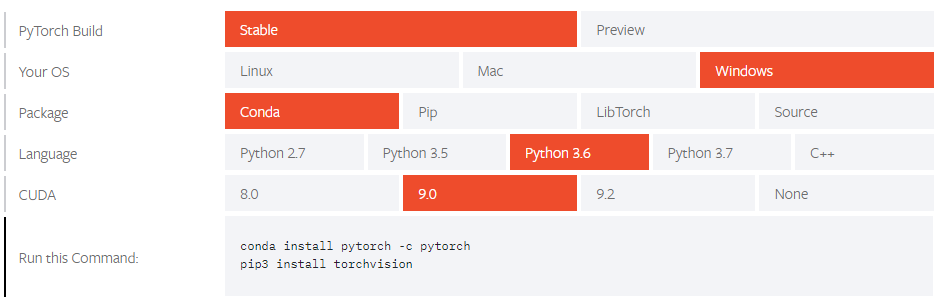
It’s pretty straight-forward based on the system properties such as the Operating System or the package managers. It can be installed from the Command Prompt or within an IDE such as PyCharm etc.
Next up on this PyTorch Tutorial blog, let us check out how NumPy is integrated into PyTorch.
Tensors are similar to NumPy’s n dimensional arrays, with the addition being that Tensors can also be used on a GPU to accelerate computing.
Let’s construct a simple tensor and check the output. First let’s check out on how we can construct a 5×3 matrix which is uninitiated:
x = torch.empty(5, 3)
print(x)
Output:
tensor([[8.3665e+22, 4.5580e-41, 1.6025e-03],
        [3.0763e-41, 0.0000e+00, 0.0000e+00],
        [0.0000e+00, 0.0000e+00, 3.4438e-41],
        [0.0000e+00, 4.8901e-36, 2.8026e-45],
        [6.6121e+31, 0.0000e+00, 9.1084e-44]])
Now let’s construct a randomly initialized matrix:
    x = torch.rand(5, 3)
    print(x)
Output:
tensor([[0.1607, 0.0298, 0.7555],
        [0.8887, 0.1625, 0.6643],
        [0.7328, 0.5419, 0.6686],
        [0.0793, 0.1133, 0.5956],
        [0.3149, 0.9995, 0.6372]])
Construct a tensor directly from data:
x = torch.tensor([5.5, 3])
print(x)
Output:
tensor([5.5000, 3.0000])Tensor Operations
There are multiple syntaxes for operations. In the following example, we will take a look at the addition operation:
y = torch.rand(5, 3)
print(x + y)
Output:
    tensor([[ 0.2349, -0.0427, -0.5053],
            [ 0.6455,  0.1199,  0.4239],
            [ 0.1279,  0.1105,  1.4637],
            [ 0.4259, -0.0763, -0.9671],
            [ 0.6856,  0.5047,  0.4250]])
Resizing: If you want to reshape/resize a tensor, you can use “torch.view”:
x = torch.randn(4, 4)
y = x.view(16)
z = x.view(-1, 8) # the size -1 is inferred from other dimensions
print(x.size(), y.size(), z.size())
Output:
torch.Size([4, 4]) torch.Size([16]) torch.Size([2, 8])![]()
NumPy is a library for the Python programming language, adding support for large, multi-dimensional arrays and matrices, along with a large collection of high-level mathematical functions to operate on these arrays.
It is also used as:
Besides its obvious scientific uses, NumPy can also be used as an efficient multi-dimensional container of generic data and arbitrary data-types can be defined as well.
This allows NumPy to seamlessly and speedily integrate with a wide variety of databases!

Converting a Torch Tensor to a NumPy array and vice versa is a breeze!
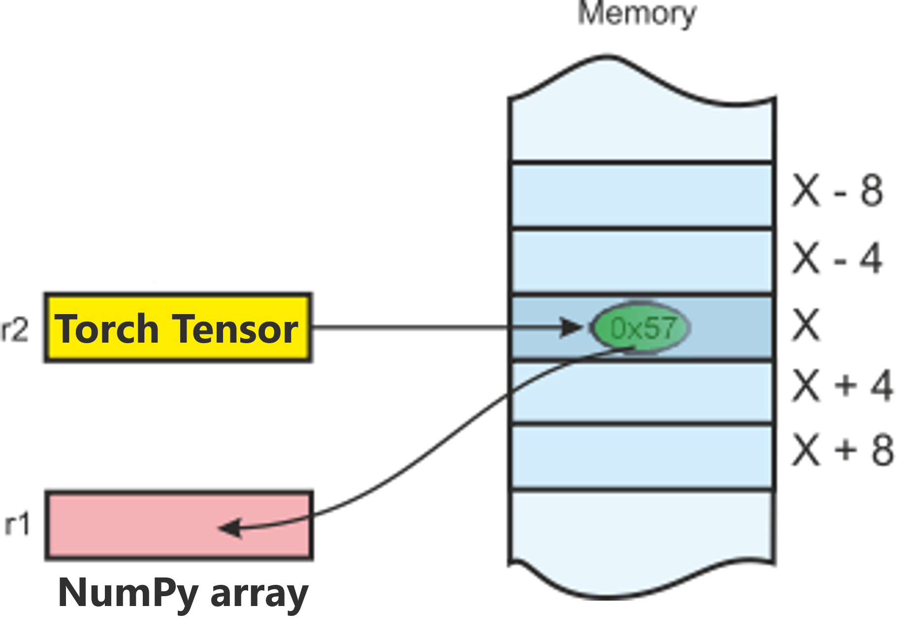
The Torch Tensor and NumPy array will share their underlying memory locations and changing one will change the other.
a = torch.ones(5)
print(a)
Output: tensor([1., 1., 1., 1., 1.])
b = a.numpy()
print(b)
Output: [1. 1. 1. 1. 1.]Let’s perform a sum operation and check the changes in the values:
a.add_(1)
print(a)
print(b)
Output: tensor([2., 2., 2., 2., 2.]) [2. 2. 2. 2. 2.]import numpy as no a = np.ones(5) b = torch.from_numpy(a) np.add(a, 1, out=a) print(a) print(b)
Output:
[2. 2. 2. 2. 2.]
tensor([2., 2., 2., 2., 2.], dtype=torch.float64)
So, as you can see, it is as simple as that!
Next up on this PyTorch Tutorial blog, let’s check out the AutoGrad module of PyTorch.
The autograd package provides automatic differentiation for all operations on Tensors.

It is a define-by-run framework, which means that your backprop is defined by how your code is run, and that every single iteration can be different.
Next up on this PyTorch Tutorial Blog, let’s look an interesting and a simple use case.
Generally, when you have to deal with image, text, audio or video data, you can use standard python packages that load data into a Numpy array. Then you can convert this array into a torch.*Tensor.
Specifically for vision, there is a package called torchvision, that has data loaders for common datasets such as Imagenet, CIFAR10, MNIST, etc. and data transformers for images.
This provides a huge convenience and avoids writing boilerplate code.
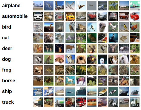
For this tutorial, we will use the CIFAR10 dataset.
It has the classes: ‘airplane’, ‘automobile’, ‘bird’, ‘cat’, ‘deer’, ‘dog’, ‘frog’, ‘horse’, ‘ship’, ‘truck’. The images in CIFAR-10 are of size 3x32x32, i.e. 3-channel color images of 32×32 pixels in size as shown below:
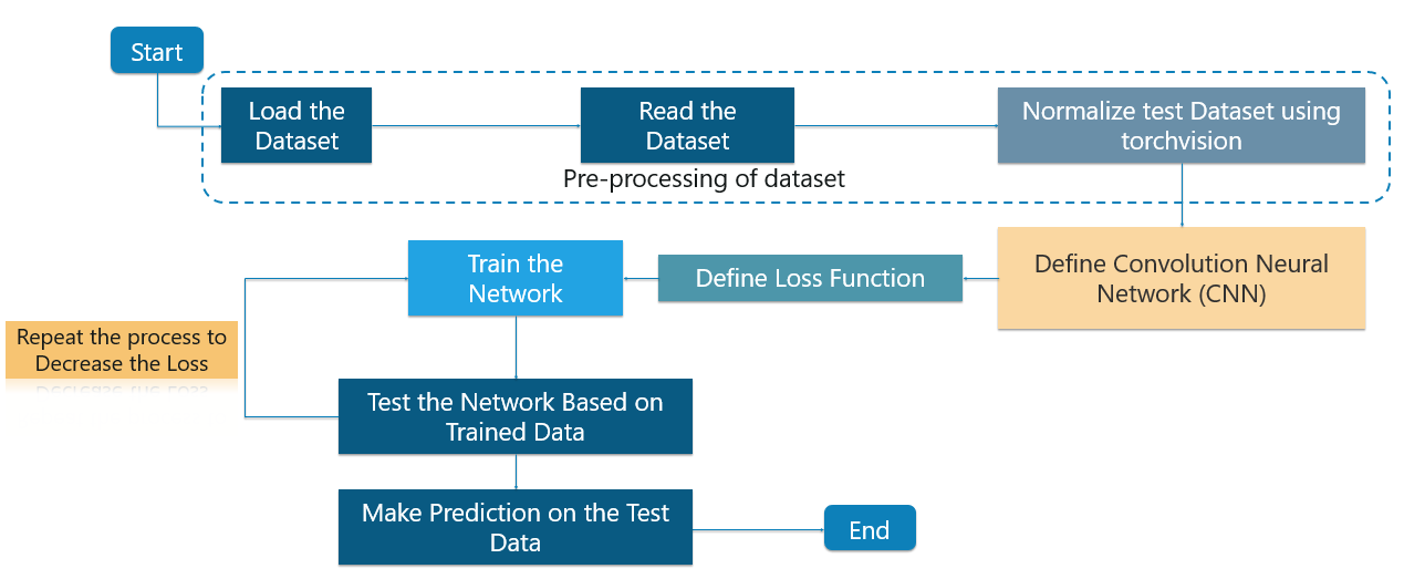
We will do the following steps in order:
Using torchvision, it is very easy to load CIFAR10!
It is as simple as follows:
import torch
import torchvision
import torchvision.transforms as transforms
The output of torchvision datasets are PILImage images of range [0, 1]. We transform them to Tensors of normalized range [-1, 1].
transform = transforms.Compose(
[transforms.ToTensor(),
transforms.Normalize((0.5, 0.5, 0.5), (0.5, 0.5, 0.5))])
trainset = torchvision.datasets.CIFAR10(root='./data', train=True,
download=True, transform=transform)
trainloader = torch.utils.data.DataLoader(trainset, batch_size=4,
shuffle=True, num_workers=2)
testset = torchvision.datasets.CIFAR10(root='./data', train=False,
download=True, transform=transform)
testloader = torch.utils.data.DataLoader(testset, batch_size=4,
shuffle=False, num_workers=2)
classes = ('plane', 'car', 'bird', 'cat',
'deer', 'dog', 'frog', 'horse', 'ship', 'truck')
Output:
Downloading https://www.cs.toronto.edu/~kriz/cifar-10-python.tar.gz to ./data/cifar-10-python.tar.gz Files already downloaded and verified Next, let us print some training images from the dataset!
import matplotlib.pyplot as plt
import numpy as np

# functions to show an image


def imshow(img):
img = img / 2 + 0.5 # unnormalize
npimg = img.numpy()
plt.imshow(np.transpose(npimg, (1, 2, 0)))


# get some random training images
dataiter = iter(trainloader)
images, labels = dataiter.next()

# show images
imshow(torchvision.utils.make_grid(images))
# print labels
print(' '.join('%5s' % classes[labels[j]] for j in range(4)))
Output:
dog bird horse horseConsider the case to use 3-channel images (Red, Green and Blue). Here’s the code to define the architecture of the CNN:
import torch.nn as nn
import torch.nn.functional as F


class Net(nn.Module):
def __init__(self):
super(Net, self).__init__()
self.conv1 = nn.Conv2d(3, 6, 5)
self.pool = nn.MaxPool2d(2, 2)
self.conv2 = nn.Conv2d(6, 16, 5)
self.fc1 = nn.Linear(16 * 5 * 5, 120)
self.fc2 = nn.Linear(120, 84)
self.fc3 = nn.Linear(84, 10)

def forward(self, x):
x = self.pool(F.relu(self.conv1(x)))
x = self.pool(F.relu(self.conv2(x)))
x = x.view(-1, 16 * 5 * 5)
x = F.relu(self.fc1(x))
x = F.relu(self.fc2(x))
x = self.fc3(x)
return x


net = Net()
We will need to define the loss function. In this case we can make use of a Classification Cross-Entropy loss. We’ll also be using SGD with momentum as well.
Basically, the Cross-Entropy Loss is a probability value ranging from 0-1. The perfect model will a Cross Entropy Loss of 0 but it might so happen that the expected value may be 0.2 but you are getting 2. This will lead to a very high loss and not be efficient at all!
import torch.optim as optim

criterion = nn.CrossEntropyLoss()
optimizer = optim.SGD(net.parameters(), lr=0.001, momentum=0.9)
This is when things start to get interesting! We simply have to loop over our data iterator, and feed the inputs to the network and optimize.
for epoch in range(2): # loop over the dataset multiple times

running_loss = 0.0
for i, data in enumerate(trainloader, 0):
# get the inputs
inputs, labels = data

# zero the parameter gradients
optimizer.zero_grad()

# forward + backward + optimize
outputs = net(inputs)
loss = criterion(outputs, labels)
loss.backward()
optimizer.step()

# print statistics
running_loss += loss.item()
if i % 2000 == 1999: # print every 2000 mini-batches
print('[%d, %5d] loss: %.3f' %
(epoch + 1, i + 1, running_loss / 2000))
running_loss = 0.0

print('Finished Training')
Output:
[1,  2000] loss: 2.236
[1,  4000] loss: 1.880
[1,  6000] loss: 1.676
[1,  8000] loss: 1.586
[1, 10000] loss: 1.515
[1, 12000] loss: 1.464
[2,  2000] loss: 1.410
[2,  4000] loss: 1.360
[2,  6000] loss: 1.360
[2,  8000] loss: 1.325
[2, 10000] loss: 1.312
[2, 12000] loss: 1.302
Finished TrainingWe have trained the network for 2 passes over the training dataset. But we need to check if the network has learnt anything at all.
We will check this by predicting the class label that the neural network outputs, and checking it against the ground-truth. If the prediction is correct, we add the sample to the list of correct predictions.
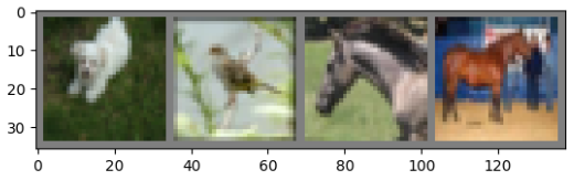
Okay, first step! Let us display an image from the test set to get familiar.
dataiter = iter(testloader)
images, labels = dataiter.next()

# print images
imshow(torchvision.utils.make_grid(images))
print('GroundTruth: ', ' '.join('%5s' % classes[labels[j]] for j in range(4)))
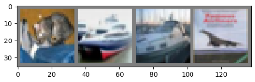
Output:
GroundTruth: cat ship ship plane
Okay, now let us see what the Neural Network thinks these examples above are:
outputs = net(images)
The outputs are energies for the 10 classes. Higher the energy for a class, the more the network thinks that the image is of the particular class. So, let’s get the index of the highest energy:
predicted = torch.max(outputs, 1)

print('Predicted: ', ' '.join('%5s' % classes[predicted[j]]
for j in range(4)))
Output:
Predicted: cat car car planeThe results seem pretty good.
Next up on this PyTorch Tutorial blog, let us look at how the network performs on the whole dataset!
correct = 0
total = 0
with torch.no_grad():
for data in testloader:
images, labels = data
outputs = net(images)
_, predicted = torch.max(outputs.data, 1)
total += labels.size(0)
correct += (predicted == labels).sum().item()

print('Accuracy of the network on the 10000 test images: %d %%' % (
100 * correct / total))
Output:
Accuracy of the network on the 10000 test images: 54 %
That looks better than chance, which is 10% accuracy (randomly picking a class out of 10 classes).
Seems like the network learned something!
What are the classes that performed well, and the classes that did not perform well?
class_correct = list(0. for i in range(10))
class_total = list(0. for i in range(10))
with torch.no_grad():
for data in testloader:
images, labels = data
outputs = net(images)
_, predicted = torch.max(outputs, 1)
c = (predicted == labels).squeeze()
for i in range(4):
label = labels[i]
class_correct[label] += c[i].item()
class_total[label] += 1


for i in range(10):
print('Accuracy of %5s : %2d %%' % (
classes[i], 100 * class_correct[i] / class_total[i]))
Output:
Accuracy of plane : 61 %
Accuracy of   car : 85 %
Accuracy of  bird : 46 %
Accuracy of   cat : 23 %
Accuracy of  deer : 40 %
Accuracy of   dog : 36 %
Accuracy of  frog : 80 %
Accuracy of horse : 59 %
Accuracy of  ship : 65 %
Accuracy of truck : 46 %
In this PyTorch Tutorial blog, we made sure to train a small Neural Network which classifies images and it turned out perfectly as expected!
Check out these interesting blogs on the following topics:
Check out this Artificial Intelligence Course with Python training by Edureka to upgrade your AI skills to the next levelYou may go through this PyTorch Tutorial video where I have explained the topics in a detailed manner with use cases that will help you to understand this concept better.
This video will help you in understanding various important basics of PyTorch.


 Thank you for registering Join Edureka Meetup community for 100+ Free Webinars each month JOIN MEETUP GROUP