Python Pandas Tutorial : Learn Pandas for Data Analysis

In this blog on ‘Python Pandas Tutorial’, we will dive deep into data analytics using the Pandas library in Python. Python Programming is a skill trending over other more prominent programming languages like Java, C++, and C#. But before we talk about Pandas, let’s start by understanding the concept of NumPy arrays. Why? Because Pandas is an open-source software library built on top of NumPy.

To get in-depth knowledge on python along with its various applications, you can enroll for live Python online course by Edureka with 24/7 support and lifetime access.

In this Python Pandas Tutorial, I will take you through the following topics, which will serve as fundamentals for the upcoming blogs:

• What is Pandas?
• Pandas Operation
  • Slicing the data frame
  • Merging & Joining
  • Concatenation
  • Changing the index
  • Change Column headers
  • Data munging
• Use-Case: Analyze youth unemployment data

Let’s get started. :-)

What is Python Pandas?

Pandas is a library in Python that is used for data manipulation, data analysis and data cleaning. Python Pandas is well suited for different kinds of data, such as 

• Tabular data with heterogeneously-typed columns
• Ordered and unordered time series data
• Arbitrary matrix data with row & column labels
• Unlabelled data
• Any other form of observational or statistical data sets

How to install Pandas?

To install Pandas in Python, you will need to open your command prompt(terminal in Linux or macOS) and type “pip install pandas”(don’t copy the quotes!)

Alternatively, if you have the Anaconda distribution installed in your system, you can type “conda install pandas”. Once the installation is completed, you can verify the installation by heading over to your preferred IDE (Jupyter, PyCharm etc.) and importing the library in your code by typing: “import pandas”. If it executes without any error, then the installation is successful. If you face a problem, you can refer to this video over here:

Python Pandas Tutorial | Pandas Library – Python Programming | Python Tutorial | Edureka

Moving ahead with our Python Pandas blog, let us take a look at some of its operations.

Python Pandas Operations

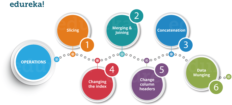
With Pandas in python, you can perform several operations with NumPy series, data frames, correction of missing data, group by operations etc.. Some of the common operations for data manipulation are listed below:

Now, let us understand all these operations one by one.

Slicing the Data Frame

The first requirement for you over here is to have access to a data frame! Now don’t worry if you don’t know what a data frame is. A data frame is just a 2-dimensional data structure and one of the most common variations of a pandas object. So first, let’s get started by creating a data frame.

Refer to the below code for the implementation of data frames

import pandas as pd

XYZ_web= {'Day':[1,2,3,4,5,6], "Visitors":[1000, 700,6000,1000,400,350], "Bounce_Rate":[20,20, 23,15,10,34]}

df= pd.DataFrame(XYZ_web)

print(df)

Output:

     Bounce_Rate Day Visitors
0     20          1   1000
1     20          2   700
2     23          3   6000
3     15          4   1000
4     10          5   400
5     34          6   350

The code above will convert a dictionary into a pandas Data Frame along with an index to the left. Now, let us slice a particular column from this data frame.

 Refer to the image below for a more accurate understanding:

print(df.head(2))

Output:

     Bounce_Rate Day Visitors
0      20         1   1000
1      20         2    700

Similarly, if you want the last two rows of the data, type in the below command:

print(df.tail(2))

Output:

  Bounce_Rate Day Visitors 
4      10      5    400
5      34      6    350

Next up in our Python Pandas tutorial, are the operations – merging and joining.

Merging & Joining

In merging, you can merge two or more data frames to form a single data frame. You can also decide and filter the columns that you want to keep common. Let me show you how to implement that practically. First I will create three data frames, which have some key-value pairs, and then merge the data frames together. Refer to the code below:

   HPI   IND_GDP Int_Rate
0  80      50      2
1  90      45      1
2  70      45      2
3  60      67      3

Output:

import pandas as pd

df1= pd.DataFrame({ "HPI":[80,90,70,60],"Int_Rate":[2,1,2,3],"IND_GDP":[50,45,45,67]}, index=[2001, 2002,2003,2004])

df2=pd.DataFrame({ "HPI":[80,90,70,60],"Int_Rate":[2,1,2,3],"IND_GDP":[50,45,45,67]}, index=[2005, 2006,2007,2008])

merged= pd.merge(df1,df2)

print(merged)

As you can see above, the two data frames has merged into a single data frame. Now, you can also specify the column which you want to make common. For example, I want the “HPI” column to be common and for everything else, I want separate columns. So, let me implement that practically:

df1 = pd.DataFrame({"HPI":[80,90,70,60],"Int_Rate":[2,1,2,3], "IND_GDP":[50,45,45,67]}, index=[2001, 2002,2003,2004])

df2 = pd.DataFrame({"HPI":[80,90,70,60],"Int_Rate":[2,1,2,3],"IND_GDP":[50,45,45,67]}, index=[2005, 2006,2007,2008])

merged= pd.merge(df1,df2,on ="HPI")

print(merged)

Output:

      IND_GDP  Int_Rate  Low_Tier_HPI  Unemployment
2001     50      2         50.0            1.0
2002     45      1         NaN             NaN
2003     45      2         45.0            3.0
2004     67      3         67.0            5.0
2004     67      3         34.0            6.0

Next up, let us understand how joining works in our Python Pandas tutorial. This is another convenient method to combine two differently indexed data frames into a single resultant data frame. This operation is quite similar to the “merge” operation that we saw before, The only difference is that the ‘joining’ operation will be on the “index” instead of the “columns”. Again, let us see this with a demonstration.

df1 = pd.DataFrame({"Int_Rate":[2,1,2,3], "IND_GDP":[50,45,45,67]}, index=[2001, 2002,2003,2004])

df2 = pd.DataFrame({"Low_Tier_HPI":[50,45,67,34],"Unemployment":[1,3,5,6]}, index=[2001, 2003,2004,2004])

joined= df1.join(df2)
print(joined)

Output:

       IND_GDP  Int_Rate Low_Tier_HPI  Unemployment
2001     50       2         50.0           1.0
2002     45       1         NaN            NaN
2003     45       2         45.0           3.0
2004     67       3         67.0           5.0
2004     67       3         34.0           6.0

As you might notice, in the year 2002(index), there is no value attached to columns “low_tier_HPI” and “unemployment”, therefore it has printed NaN (Not a Number). Later in 2004, both of these values are available, The function accurately modified the data frame

You may go through this recording of Python Pandas tutorial where our instructor has explained the topics in a detailed manner with examples that will help you to understand this concept better.

Python For Data Analysis | Python Pandas Tutorial | Python Training | Edureka

Moving ahead with our Python Pandas tutorial, let’s understand how to concatenate two data frames. This operation is called concatenation. 

Concatenation 

This operation basically glues the dataframes together. You can select the dimension on which you want to concatenate. For that, just use “pd.concat” and pass in the list of dataframes to concatenate together. Consider the below example.

df1 = pd.DataFrame({"HPI":[80,90,70,60],"Int_Rate":[2,1,2,3], "IND_GDP":[50,45,45,67]}, index=[2001, 2002,2003,2004])

df2 = pd.DataFrame({"HPI":[80,90,70,60],"Int_Rate":[2,1,2,3],"IND_GDP":[50,45,45,67]}, index=[2005, 2006,2007,2008])

concat= pd.concat([df1,df2])

print(concat)

Output:

       HPI  IND_GDP Int_Rate
2001    80    50       2
2002    90    45       1
2003    70    45       2
2004    60    67       3
2005    80    50       2
2006    90    45       1
2007    70    45       2
2008    60    67       3

As you can see above, the two dataframes are glued together in a single data frame, where the index starts from 2001 all the way up to 2008. Next, you can also specify a parameter: `axis=1` in order to join, merge or concatenate along the columns. For this, you can refer to the code below:

df1 = pd.DataFrame({"HPI":[80,90,70,60],"Int_Rate":[2,1,2,3], "IND_GDP":[50,45,45,67]}, index=[2001, 2002,2003,2004])

df2 = pd.DataFrame({"HPI":[80,90,70,60],"Int_Rate":[2,1,2,3],"IND_GDP":[50,45,45,67]}, index=[2005, 2006,2007,2008])

concat= pd.concat([df1,df2],axis=1)

print(concat)

Output:

       HPI  IND_GDP  Int_Rate HPI  IND_GDP Int_Rate
2001   80.0  50.0       2.0   NaN    NaN     NaN
2002   90.0  45.0       1.0   NaN    NaN     NaN
2003   70.0  45.0       2.0   NaN    NaN     NaN
2004   60.0  67.0       3.0   NaN    NaN     NaN
2005   NaN   NaN        NaN   80.0   50.0    2.0
2006   NaN   NaN        NaN   90.0   45.0    1.0
2007   NaN   NaN        NaN   70.0   45.0    2.0
2008   NaN   NaN        NaN   60.0   67.0    3.0

If you observe the values listed above, there are a bunch of missing values. This happens because the data frames didn’t have values for all the indexes you want to concatenate on. Therefore, you should make sure that you have all the information lining up correctly when you join or concatenate on the axis.

Changing the index

Up next in our Python Pandas tutorial, we’ll understand how to change the index values in a data frame. For example, let us create a data frame with some key-value pairs in a dictionary and change the index values. Consider the example below:

Let us see how it actually happens:

import pandas as pd

df= pd.DataFrame({"Day":[1,2,3,4], "Visitors":[200, 100,230,300], "Bounce_Rate":[20,45,60,10]}) 

df.set_index("Day", inplace= True)

print(df)

Output:

     Bounce_Rate  Visitors
Day 
1      20           200
2      45           100
3      60           230
4      10           300

As you can notice in the output above, the index value has been changed with respect to the “Day” column.

Changing the Column Headers

We’ll now see how to change the headers of a column(s) in this Python Pandas tutorial. Let us take the same example, where I will change the column header from “Visitors” to “Users”. So, let me implement it practically.

import pandas as pd

df = pd.DataFrame({"Day":[1,2,3,4], "Visitors":[200, 100,230,300], "Bounce_Rate":[20,45,60,10]})

df = df.rename(columns={"Visitors":"Users"})

print(df)

Output:

  Bounce_Rate  Day  Users
0    20         1    200
1    45         2    100
2    60         3    230
3    10         4    300

As you see above, column header “Visitors” has been changed to “Users”. Next in the python pandas tutorial, let us perform data munging.

Data Munging

In Data munging, you can convert a particular data into a different format. For example, if you have a .csv file, you can convert it into .html  You can convert it into any other data format as well. 

import pandas as pd

country= pd.read_csv("D:UsersAayushiDownloadsworld-bank-youth-unemploymentAPI_ILO_country_YU.csv",index_col=0)

country.to_html('edu.html')

Once you run this code, an HTML file will be created named “edu.html”. You can directly copy the path of the file and paste it in your browser which displays the data in a HTML format. Refer the below screenshot:

Next in the python pandas tutorial, let’s have a look at a use-case that talks about global youth unemployment.

Python Pandas Tutorial: Use Case to Analyze Youth Unemployment Data

Problem Statement: You are given a dataset that comprises the percentage of unemployed youth globally from 2010 to 2014. You have to use this dataset and find the change in the percentage of youth for every country from 2010-2011.

First, let us understand the dataset which contains the columns as Country Name, Country Code, and the year from 2010 to 2014. Now using pandas, We’ll read the .csv file using the snippet “pd.read_csv”. Refer the screenshot below:

Let us move ahead and perform data analysis here we are going to find out the difference in percentile among the unemployed youth between 2010 to 2011. Then we will visualize the same using the Matplotlib library, which is a powerful library for visualization in Python. It can be used in Python scripts, shell, web application servers and other GUI toolkits. You can use read more here: Matplotlib Tutorial.

Now, let us implement the code in PyCharm:

import pandas as pd

import matplotlib.pyplot as plt

from matplotlib import style

style.use('fivethirtyeight')

country= pd.read_csv("D:UsersAayushiDownloadsworld-bank-youth-unemploymentAPI_ILO_country_YU.csv",index_col=0)

df= country.head(5)

df= df.set_index(["Country Code"])

sd = sd.reindex(columns=['2010','2011'])

db= sd.diff(axis=1)

db.plot(kind="bar")

plt.show()

As you can see above, I have performed the analysis on the top 5 rows of the country data frame. Next, I have defined an index value to be “Country Code” and then re-index the column to 2010 and 2011. Then, we have one more data frame DB, which prints the difference between the two columns or the percentage change of unemployed youth between the years 2010 to 2011. Finally, I have plotted a barplot using the Matplotlib library in Python.

Now if you noticed in the above plot, in Afghanistan(AFG) between 2010 to 2011, there has been a rise in unemployed youth of approx. 0.25%. Then in Angola(AGO), there is a negative trend which means that the percentage of unemployed youth has been reduced. You can go ahead and experiment with the data by yourself. Take a few minutes and come up with some insights. Let us know what you found in the comments!

I hope my blog on “Python Pandas Tutorial” was relevant for you.

Got a question for us? Please mention it in the comments section of this “Python Pandas tutorial” blog  and we will get back to you as soon as possible.