All You Need To Know About Principal Component Analysis (PCA)

With the advancements in the field of Machine Learning and Artificial Intelligence, it has become essential to understand the fundamentals behind such technologies. This blog on Principal Component Analysis will help you understand the concepts behind dimensionality reduction and how it can be used to deal with high dimensional data.

To get in-depth knowledge of Artificial Intelligence and Machine Learning, you can enroll for live Machine Learning Engineer Master Program by Edureka with 24/7 support and lifetime access.

Here’s a list of topics that will be covered in this blog:

1. 1. Need For Principal Component Analysis
   2. What is PCA?
   3. Step by step computation of PCA
      1. Standardization
      2. Computing Covariance Matrix
      3. Calculating Eigenvector and eigenvalue
      4. Compute Principal Components
      5. Reduce data dimension
   4. Principal Component Analysis With Python

Need For Principal Component Analysis (PCA)

Machine Learning in general works wonders when the dataset provided for training the machine is large and concise. Usually having a good amount of data lets us build a better predictive model since we have more data to train the machine with. However, using a large data set has its own pitfalls. The biggest pitfall is the curse of dimensionality.

It turns out that in large dimensional datasets, there might be lots of inconsistencies in the features or lots of redundant features in the dataset, which will only increase the computation time and make data processing and EDA more convoluted.

To get rid of the curse of dimensionality, a process called dimensionality reduction was introduced. Dimensionality reduction techniques can be used to filter only a limited number of significant features needed for training and this is where PCA comes in.

What Is Principal Component Analysis (PCA)? 

Principal components analysis (PCA) is a dimensionality reduction technique that enables you to identify correlations and patterns in a data set so that it can be transformed into a data set of significantly lower dimension without loss of any important information.

The main idea behind PCA is to figure out patterns and correlations among various features in the data set. On finding a strong correlation between different variables, a final decision is made about reducing the dimensions of the data in such a way that the significant data is still retained.

Such a process is very essential in solving complex data-driven problems that involve the use of high-dimensional data sets. PCA can be achieved via a series of steps. Let’s discuss the whole end-to-end process.

Step By Step Computation Of PCA

The below steps need to be followed to perform dimensionality reduction using PCA:

1. Standardization of the data
2. Computing the covariance matrix
3. Calculating the eigenvectors and eigenvalues
4. Computing the Principal Components
5. Reducing the dimensions of the data set

Let’s discuss each of the steps in detail:

Step 1: Standardization of the data

If you’re familiar with data analysis and processing, you know that missing out on standardization will probably result in a biased outcome. Standardization is all about scaling your data in such a way that all the variables and their values lie within a similar range.

Consider an example, let’s say that we have 2 variables in our data set, one has values ranging between 10-100 and the other has values between 1000-5000. In such a scenario, it is obvious that the output calculated by using these predictor variables is going to be biased since the variable with a larger range will have a more obvious impact on the outcome.

Therefore, standardizing the data into a comparable range is very important. Standardization is carried out by subtracting each value in the data from the mean and dividing it by the overall deviation in the data set.

It can be calculated like so:

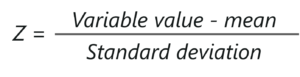Post this step, all the variables in the data are scaled across a standard and comparable scale.

Step 2: Computing the covariance matrix

As mentioned earlier, PCA helps to identify the correlation and dependencies among the features in a data set. A covariance matrix expresses the correlation between the different variables in the data set. It is essential to identify heavily dependent variables because they contain biased and redundant information which reduces the overall performance of the model.

Mathematically, a covariance matrix is a p × p matrix, where p represents the dimensions of the data set. Each entry in the matrix represents the covariance of the corresponding variables.

Consider a case where we have a  2-Dimensional data set with variables a and b, the covariance matrix is a 2×2 matrix as shown below:

In the above matrix:

• Cov(a, a) represents the covariance of a variable with itself, which is nothing but the variance of the variable ‘a’
• Cov(a, b) represents the covariance of the variable ‘a’ with respect to the variable ‘b’. And since covariance is commutative, Cov(a, b) = Cov(b, a)

Here are the key takeaways from the covariance matrix:

• The covariance value denotes how co-dependent two variables are with respect to each other
• If the covariance value is negative, it denotes the respective variables are indirectly proportional to each other
• A positive covariance denotes that the respective variables are directly proportional to each other

Simple math, isn’t it? Now let’s move on and look at the next step in PCA.

Step 3: Calculating the Eigenvectors and Eigenvalues

Eigenvectors and eigenvalues are the mathematical constructs that must be computed from the covariance matrix in order to determine the principal components of the data set.

But first, let’s understand more about principal components

What are Principal Components?

Simply put, principal components are the new set of variables that are obtained from the initial set of variables. The principal components are computed in such a manner that newly obtained variables are highly significant and independent of each other. The principal components compress and possess most of the useful information that was scattered among the initial variables.

If your data set is of 5 dimensions, then 5 principal components are computed, such that, the first principal component stores the maximum possible information and the second one stores the remaining maximum info and so on, you get the idea.

Now, where do Eigenvectors fall into this whole process?

Assuming that you all have a basic understanding of Eigenvectors and eigenvalues, we know that these two algebraic formulations are always computed as a pair, i.e, for every eigenvector there is an eigenvalue. The dimensions in the data determine the number of eigenvectors that you need to calculate.

Consider a 2-Dimensional data set, for which 2 eigenvectors (and their respective eigenvalues) are computed. The idea behind eigenvectors is to use the Covariance matrix to understand where in the data there is the most amount of variance. Since more variance in the data denotes more information about the data, eigenvectors are used to identify and compute Principal Components.

Eigenvalues, on the other hand, simply denote the scalars of the respective eigenvectors. Therefore, eigenvectors and eigenvalues will compute the Principal Components of the data set.

Step 4: Computing the Principal Components

Once we have computed the Eigenvectors and eigenvalues, all we have to do is order them in the descending order, where the eigenvector with the highest eigenvalue is the most significant and thus forms the first principal component. The principal components of lesser significances can thus be removed in order to reduce the dimensions of the data.

The final step in computing the Principal Components is to form a matrix known as the feature matrix that contains all the significant data variables that possess maximum information about the data.

Step 5: Reducing the dimensions of the data set

The last step in performing PCA is to re-arrange the original data with the final principal components which represent the maximum and the most significant information of the data set. In order to replace the original data axis with the newly formed Principal Components, you simply multiply the transpose of the original data set by the transpose of the obtained feature vector.

So that was the theory behind the entire PCA process. It’s time to get your hands dirty and perform all these steps by using a real data set.

Principal Component Analysis Using Python

In this section, we will be performing PCA by using Python. If you’re not familiar with the Python programming language, give these blogs a read:

1. Python Tutorial – A Complete Guide to Learn Python Programming
2. Python Programming Language – Headstart With Python Basics
3. A Beginners Guide To Python Functions
4. Python for Data Science

Problem Statement: To perform step by step Principal Component Analysis in order to reduce the dimension of the data set.

Data set Description: Movies rating data set that contains ratings from 700+ users for approximately 9000 movies (features).

Logic: Perform PCA by finding the most significant features in the data. PCA will be performed by following the steps that were defined above.

Let’s get started!

Step 1: Import required packages

import pandas as pd
import numpy as np
from sklearn.preprocessing import StandardScaler
from matplotlib import*
import matplotlib.pyplot as plt
from matplotlib.cm import register_cmap
from scipy import stats
from sklearn.decomposition import PCA as sklearnPCA
import seaborn

Step 2: Import data set

#Load movie names and movie ratings
movies = pd.read_csv('C:UsersNeelTempDesktopPCA DATAmovies.csv')
ratings = pd.read_csv('C:UsersNeelTempDesktopPCA DATAratings.csv')
ratings.drop(['timestamp'], axis=1, inplace=True)

Step 3: Formatting the data

def replace_name(x):
return movies[movies['movieId']==x].title.values[0]
ratings.movieId = ratings.movieId.map(replace_name)
M = ratings.pivot_table(index=['userId'], columns=['movieId'], values='rating')
m = M.shape
df1 = M.replace(np.nan, 0, regex=True)

Step 4: Standardization

In the below line of code, we use the StandardScalar() function provided by the sklearn package in order to scale the data set within comparable ranges. As discussed earlier, standardization is required to prevent biases in the final outcome.

X_std = StandardScaler().fit_transform(df1)

Step 5: Compute covariance matrix

As discussed earlier, a covariance matrix expresses the correlation between the different features in the data set. It is essential to identify heavily dependent variables because they contain biased and redundant information which reduces the overall performance of the model. The below code snippet computes the covariance matrix for the data:

mean_vec = np.mean(X_std, axis=0)
cov_mat = (X_std - mean_vec).T.dot((X_std - mean_vec)) / (X_std.shape[0]-1)
print('Covariance matrix n%s' %cov_mat)

Covariance matrix
[[ 1.0013947 -0.00276421 -0.00195661 ... -0.00858289 -0.00321221
-0.01055463]
[-0.00276421 1.0013947 -0.00197311 ... 0.14004611 -0.0032393
-0.01064364]
[-0.00195661 -0.00197311 1.0013947 ... -0.00612653 -0.0022929
-0.00753398]
...
[-0.00858289 0.14004611 -0.00612653 ... 1.0013947 0.02888777
0.14005644]
[-0.00321221 -0.0032393 -0.0022929 ... 0.02888777 1.0013947
0.01676203]
[-0.01055463 -0.01064364 -0.00753398 ... 0.14005644 0.01676203
1.0013947 ]]

Step 6: Calculate eigenvectors and eigenvalues

In this step eigenvectors and eigenvalues are calculated which basically compute the Principal Components of the data set.

#Calculating eigenvectors and eigenvalues on covariance matrix
cov_mat = np.cov(X_std.T)
eig_vals, eig_vecs = np.linalg.eig(cov_mat)
print('Eigenvectors n%s' %eig_vecs)
print('nEigenvalues n%s' %eig_vals)

Eigenvectors
[[-1.34830861e-04+0.j 5.76715196e-04+0.j 4.83014783e-05+0.j ...
5.02355418e-14+0.j 6.48472777e-12+0.j 6.90776605e-13+0.j]
[ 5.61303451e-04+0.j -1.11493526e-02+0.j 8.85798170e-03+0.j ...
-2.38204858e-11+0.j -6.11345049e-11+0.j -1.39454110e-12+0.j]
[ 4.58686517e-04+0.j -2.39083484e-03+0.j 6.58309436e-04+0.j ...
-7.00290160e-12+0.j -5.53245120e-12+0.j 3.35918400e-13+0.j]
...
[ 5.22202072e-03+0.j -5.49944367e-03+0.j 5.16164779e-03+0.j ...
2.53271844e-10+0.j 9.69246536e-10+0.j 5.86126443e-11+0.j]
[ 8.97514078e-04+0.j -1.14918748e-02+0.j 9.41277803e-03+0.j ...
-3.90405498e-10+0.j -7.88691586e-10+0.j -2.80604702e-11+0.j]
[ 4.36362199e-03+0.j -7.90241494e-03+0.j -7.48537922e-03+0.j ...
-6.38353830e-10+0.j -6.47370973e-10+0.j 1.41147483e-13+0.j]]

Eigenvalues
[ 1.54166656e+03+0.j 4.23920460e+02+0.j 3.19074475e+02+0.j ...
8.84301723e-64+0.j 1.48644623e-64+0.j -3.46531190e-65+0.j]

Step 7: Compute the feature vector 

In this step, we rearrange the eigenvalues in descending order. This represents the significance of the principal components in descending order:

# Visually confirm that the list is correctly sorted by decreasing eigenvalues
eig_pairs = [(np.abs(eig_vals[i]), eig_vecs[:,i]) for i in range(len(eig_vals))]
print('Eigenvalues in descending order:')
for i in eig_pairs:
print(i[0])

Eigenvalues in descending order:
1541.6665576008295
423.92045998539083
319.07447507743535
279.33035758081536
251.63844082955103
218.62439973216058
154.61586911307694
138.60396745179094
137.6669785626203
119.37014654115806
115.2795566625854
105.40594030056845
97.84201186745533
96.72012660587329
93.39647211318346
87.7491937345281
87.54664687999116
85.93371257360843
72.85051428001277
70.37154679336622
64.45310203297905
63.78603164551922
62.11260590665646
60.080661628776205
57.67255079811343
56.490104252992744
55.48183563193681
53.78161965096411

....

Step 8: Use the PCA() function to reduce the dimensionality of the data set

The below code snippet uses the pre-defined PCA() function provided by the sklearn package in order to transform the data. The n_components parameter denotes the number of Principal Components you want to fit your data with:

pca = PCA(n_components=2)
pca.fit_transform(df1)
print(pca.explained_variance_ratio_)

[0.13379809 0.03977444]

The output shows that PC1 and PC2 account for approximately 14% of the variance in the data set.

Step 9: Projecting the variance w.r.t the Principle Components

To gain insights on the variance of the data with respect to a varied number of principal components let’s graph a scree plot. In statistics, a scree plot expresses the variance associated with each principal component:

pca = PCA().fit(X_std)
plt.plot(np.cumsum(pca.explained_variance_ratio_))
plt.xlabel('number of components')
plt.ylabel('cumulative explained variance')
plt.show()

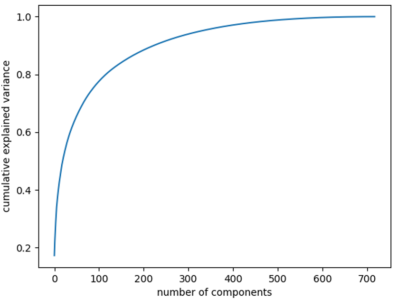The scree plot clearly indicates that the first 500 principal components contain the maximum information (variance) within the data. Note that the initial data set had approximately 9000 features which can now be narrowed down to just 500. Thus, you can now easily perform further analysis on the data since the redundant or insignificant variables are out. This is the power of dimensionality reduction.

Now that you know the math behind Principal Component Analysis, I’m sure you’re curious to learn more. Here’s a list of blogs that will help you get started with other statistical concepts:

1. A Complete Guide To Math And Statistics For Data Science
2. All You Need To Know About Statistics And Probability
3. Introduction To Markov Chains With Examples – Markov Chains With Python
4. How To Implement Bayesian Networks In Python? – Bayesian Networks Explained With Examples

With this, we come to the end of this blog. If you have any queries regarding this topic, please leave a comment below and we’ll get back to you.

If you wish to enroll for a complete course on Artificial Intelligence and Machine Learning, Edureka has a specially curated Machine Learning Engineer Master Program that will make you proficient in techniques like Supervised Learning, Unsupervised Learning, and Natural Language Processing. It includes training on the latest advancements and technical approaches in Artificial Intelligence & Machine Learning such as Deep Learning, Graphical Models and Reinforcement Learning.