Data Science with Python Certification Course
- 131k Enrolled Learners
- Weekend
- Live Class
Building a Machine Learning model is not just about feeding the data, there is a lot of deficiencies that affect the accuracy of any model. Overfitting in Machine Learning is one such deficiency in Machine Learning that hinders the accuracy as well as the performance of the model. The following topics are covered in this article:
A statistical model is said to be overfitted when we feed it a lot more data than necessary. To make it relatable, imagine trying to fit into oversized apparel.
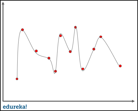
When a model fits more data than it actually needs, it starts catching the noisy data and inaccurate values in the data. As a result, the efficiency and accuracy of the model decrease. Let us take a look at a few examples of overfitting in order to understand how it actually happens.
Transform yourself into a highly skilled professional and land a high-paying job with the Artificial Intelligence Course.
Example 1
If we take an example of simple linear regression, training the data is all about finding out the minimum cost between the best fit line and the data points. It goes through a number of iterations to find out the optimum best fit, minimizing the cost. This is where overfitting comes into the picture.
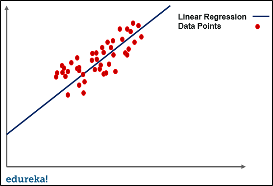
The line seen in the image above can give a very efficient outcome for a new data point. In the case of overfitting, when we run the training algorithm on the data set, we allow the cost to reduce with each number of iteration.
Running this algorithm for too long will mean a reduced cost but it will also fit the noisy data from the data set. The result would look something like in the graph below.

This might look efficient but isn’t really. The main goal of an algorithm such as linear regression is to find a dominant trend and fit the data points accordingly. But in this case, the line fits all data points, which is irrelevant to the efficiency of the model in predicting optimum outcomes for new entry data points.
Now let us consider a more descriptive example with the help of a problem statement.
Example 2
Problem Statement: Let us consider we want to predict if a soccer player will land a slot in a tier 1 football club based on his/her current performance in the tier 2 league.
Now imagine, we train and fit the model with 10,000 such players with outcomes. When we try to predict the outcome on the original data set, let us say we got a 99% accuracy. But the accuracy on a different data set comes around 50 percent. This means the model does not generalize well from our training data and unseen data.
This is what overfitting looks like. It is a very common problem in Machine Learning and even data science. Now let us understand the signal and noise.
In predictive modeling, signal refers to the true underlying pattern that helps the model to learn the data. On the other hand, noise is irrelevant and random data in the data set. To understand the concept of noise and signal, let us take a real-life example.
Let us suppose we want to model age vs literacy among adults. If we sample a very large part of the population, we will find a clear relationship. This is the signal, whereas noise interferes with the signal. If we do the same on a local population, the relationship will become muddy. It would be affected by outliers and randomness, for e.g, one adult went to school early or some adult couldn’t afford education, etc.
Talking about noise and signal in terms of Machine Learning, a good Machine Learning algorithm will automatically separate signals from the noise. If the algorithm is too complex or inefficient, it may learn the noise too. Hence, overfitting the model. Let us also understand underfitting in Machine Learning as well.
In order to avoid overfitting, we could stop the training at an earlier stage. But it might also lead to the model not being able to learn enough from training data, that it may find it difficult to capture the dominant trend. This is known as underfitting. The result is the same as overfitting, inefficiency in predicting outcomes.
Now that we have understood what underfitting and overfitting in Machine Learning really is, let us try to understand how we can detect overfitting in Machine Learning.
The main challenge with overfitting is to estimate the accuracy of the performance of our model with new data. We would not be able to estimate the accuracy until we actually test it.
To address this problem, we can split the initial data set into separate training and test data sets. With this technique, we can actually approximate how well our model will perform with the new data.
Let us understand this with an example, imagine we get a 90+ percent accuracy on the training set and a 50 percent accuracy on the test set. Then, automatically it would be a red flag for the model.
Another way to detect overfitting is to start with a simplistic model that will serve as a benchmark.
With this approach, if you try more complex algorithms you will be able to understand if the additional complexity is even worthwhile for the model or not. It is also known as Occam’s razor test, it basically chooses the simplistic model in case of comparable performance in case of two models. Although detecting overfitting is a good practice, but there are several techniques to prevent overfitting as well. Let us take a look at how we can prevent overfitting in Machine Learning.
There are several techniques to avoid overfitting in Machine Learning altogether listed below.
One of the most powerful features to avoid/prevent overfitting is cross-validation. The idea behind this is to use the initial training data to generate mini train-test-splits, and then use these splits to tune your model.
In a standard k-fold validation, the data is partitioned into k-subsets also known as folds. After this, the algorithm is trained iteratively on k-1 folds while using the remaining folds as the test set, also known as holdout fold.
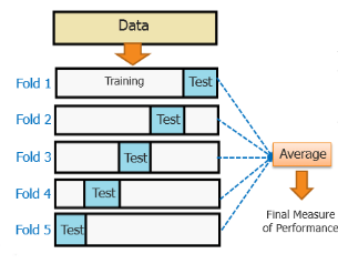 The cross-validation helps us to tune the hyperparameters with only the original training set. It basically keeps the test set separately as a true unseen data set for selecting the final model. Hence, avoiding overfitting altogether.
This technique might not work every time, as we have also discussed in the example above, where training with a significant amount of population helps the model. It basically helps the model in identifying the signal better.
But in some cases, the increased data can also mean feeding more noise to the model. When we are training the model with more data, we have to make sure the data is clean and free from randomness and inconsistencies.
Although some algorithms have an automatic selection of features. For a significant number of those who do not have a built-in feature selection, we can manually remove a few irrelevant features from the input features to improve the generalization.
One way to do it is by deriving a conclusion as to how a feature fits into the model. It is quite similar to debugging the code line-by-line.
In case if a feature is unable to explain the relevancy in the model, we can simply identify those features. We can even use a few feature selection heuristics for a good starting point.
When the model is training, you can actually measure how well the model performs based on each iteration. We can do this until a point when the iterations improve the model’s performance. After this, the model overfits the training data as the generalization weakens after each iteration.
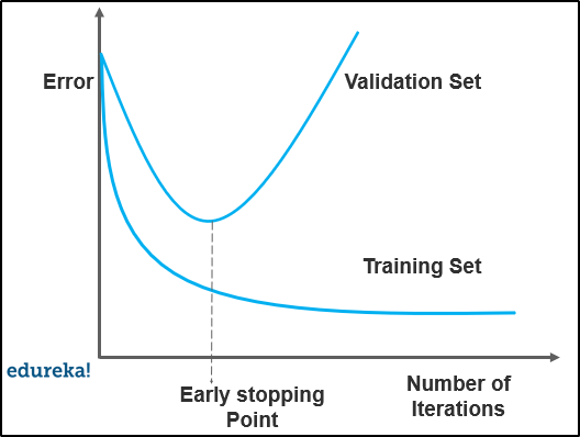
So basically, early stopping means stopping the training process before the model passes the point where the model begins to overfit the training data. This technique is mostly used in deep learning.
It basically means, artificially forcing your model to be simpler by using a broader range of techniques. It totally depends on the type of learner that we are using. For example, we can prune a decision tree, use a dropout on a neural network or add a penalty parameter to the cost function in regression.
Quite often, regularization is a hyperparameter as well. It means it can also be tuned through cross-validation.
This technique basically combines predictions from different Machine Learning models. Two of the most common methods for ensembling are listed below:
Bagging attempts to reduce the chance overfitting the models
Boosting attempts to improve the predictive flexibility of simpler models
Even though they are both ensemble methods, the approach totally starts from opposite directions. Bagging uses complex base models and tries to smooth out their predictions while boosting uses simple base models and tries to boost its aggregate complexity.
In statistic modeling, the goodness of fit refers to how closely the outcomes or predicted values match the observed or true values. A model that has learned noise instead of the signal is overfitted because it will fit the training data set but will have poorer efficiency with the new data set.
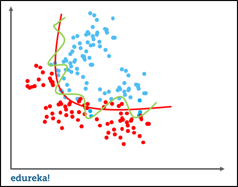
Both variance and bias are forms of prediction error in Machine Learning. The trade-off between high variance and high bias is a very important concept in statistics and Machine Learning. This is one concept that affects all the supervised Machine Learning algorithms.
The bias-variance trade-off has a very significant impact on determining the complexity, underfitting, and overfitting for any Machine Learning model.
Bias
It is nothing but the difference between the predicted values and the actual or true values in the model. It is not always easy for the model to learn from rather complex signals.
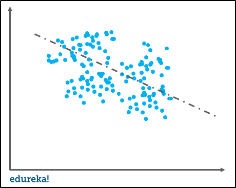
Let us imagine fitting a linear regression to a model with non-linear data. No matter how efficiently the model learns the observations, it will not model the curves efficiently. It is known as underfitting.
Variance
It refers to the model’s sensitivity to specific sets in the training data. A high variance algorithm will produce a bizarre model that is drastically different from the training set.
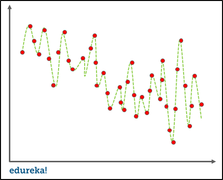
Imagine an algorithm that fits the unconstrained and super-flexible model, it will also learn from the noise in the training set causing overfitting.
Bias-Variance Trade-off
A Machine Learning algorithm cannot be perceived as a one-time method for training the model, instead, it is a repetitive process.
Low variance-high bias algorithms are less complex, with a simple and rigid structure.
They will train the models that are consistent, but inaccurate on average.
These include linear or parametric algorithms, such as regression, Naive Bayes, etc.
High variance-low bias algorithms tend to be more complex, with a flexible structure.
They will train the models that are inconsistent but accurate on average.
These include non-linear or non-parametric algorithms such as decision trees, Nearest neighbor, etc.
This brings us to the end of this article where we have learned Overfitting in Machine learning and about various techniques to avoid it. I hope you are clear with all that has been shared with you in this tutorial.
If you found this article on “Overfitting In Machine Learning” relevant, check out the Edureka’s best Machine Learning Certification Training a trusted online learning company with a network of more than 250,000 satisfied learners spread across the globe.
We are here to help you with every step on your journey and come up with a curriculum that is designed for students and professionals who want to be a Machine Learning Engineer. The course is designed to give you a head start into Python programming and train you for both core and advanced Python concepts along with various Machine learning Algorithms like SVM, Decision Tree, etc. With immense applications and easier implementations of Python with data science, there has been a significant increase in the number of jobs created for data science every year. Enroll for Edureka’s Data Science with Python Certification Course and get hands-on experience with real-time industry projects along with 24×7 support, which will set you on the path of becoming a successful Data Scientist.
If you come across any questions, feel free to ask all your questions in the comments section of “Overfitting In Machine Learning” and our team will be glad to answer.
 Thank you for registering Join Edureka Meetup community for 100+ Free Webinars each month JOIN MEETUP GROUP
edureka.co