Naive Bayes Classifier: Learning Naive Bayes with Python

In a world full of Machine Learning and Artificial Intelligence, surrounding almost everything around us, Classification and Prediction is one the most important aspects of Machine Learning and Naive Bayes is a simple but surprisingly powerful algorithm for predictive modeling according to Machine Learning Industry Experts. So Guys, in this Naive Bayes Tutorial, I’ll be covering the following topics:

• • What is Naive Bayes?
  • What is Bayes Theorem?
  • Game Prediction using Bayes’ Theorem
  • Naive Bayes in the Industry
  • Step By Step Implementation of Naive Bayes
  • Naive Bayes with SKLEARN

What is Naive Bayes? 

Naive Bayes is among one of the most simple and powerful algorithms for classification based on Bayes’ Theorem with an assumption of independence among predictors. Naive Bayes model is easy to build and particularly useful for very large data sets. There are two parts to this algorithm:

• Naive
• Bayes

The Naive Bayes classifier assumes that the presence of a feature in a class is unrelated to any other feature. Even if these features depend on each other or upon the existence of the other features, all of these properties independently contribute to the probability that a particular fruit is an apple or an orange or a banana and that is why it is known as “Naive”. 

Let’s move forward with our Naive Bayes Tutorial Blog and understand Bayes Theorem.

What is Bayes Theorem?

In Statistics and probability theory, Bayes’ theorem describes the probability of an event, based on prior knowledge of conditions that might be related to the event. It serves as a way to figure out conditional probability.

Given a Hypothesis H and evidence E, Bayes’ Theorem states that the relationship between the probability of Hypothesis before getting the evidence P(H) and the probability of the hypothesis after getting the evidence P(H|E) is :

This relates the probability of the hypothesis before getting the evidence P(H), to the probability of the hypothesis after getting the evidence, P(H|E). For this reason,  is called the prior probability, while P(H|E) is called the posterior probability. The factor that relates the two, P(H|E) / P(E), is called the likelihood ratio. Using these terms, Bayes’ theorem can be rephrased as:

“The posterior probability equals the prior probability times the likelihood ratio.”

Go a little confused? Don’t worry.
Let’s continue our Naive Bayes Tutorial blog and understand this concept with a simple concept.

Bayes’ Theorem Example

Let’s suppose we have a Deck of Cards, we wish to find out the “Probability of the Card we picked at random to be a King given that it is a Face Card“. So, according to Bayes Theorem, we can solve this problem. First, we need to find out the probability

• P(King) which is 4/52 as there are 4 Kings in a Deck of Cards.
• P(Face|King) is equal to 1 as all the Kings are face Cards.
• P(Face) is equal to 12/52 as there are 3 Face Cards in a Suit of 13 cards and there are 4 Suits in total.

Now, putting all the values in the Bayes’ Equation we get the result as 1/3

Game Prediction using Bayes’ Theorem

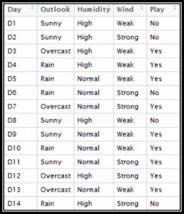
Let’s continue our Naive Bayes Tutorial blog and Predict the Future of Playing with the weather data we have.

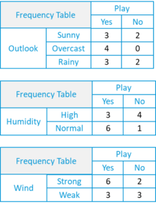
So here we have our Data, which comprises of the Day, Outlook, Humidity, Wind Conditions and the final column being Play, which we have to predict.

• First, we will create a frequency table using each attribute of the dataset.

• For each frequency table, we will generate a likelihood table.

• Likelihood of ‘Yes’ given ‘Sunny‘ is:

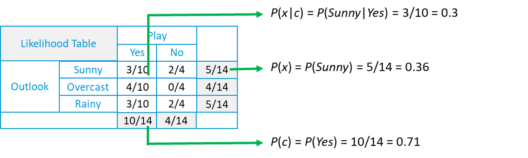
P(c|x) = P(Yes|Sunny) = P(Sunny|Yes)* P(Yes) / P(Sunny) = (0.3 x 0.71) /0.36  = 0.591

• Similarly Likelihood of ‘No’ given ‘Sunny‘ is:

P(c|x) = P(No|Sunny) = P(Sunny|No)* P(No) / P(Sunny) = (0.4 x 0.36) /0.36  = 0.40

• Now, in the same way, we need to create the Likelihood Table for other attributes as well.

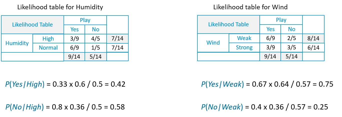
Suppose we have a Day with the following values :

• Outlook   =  Rain
• Humidity   =  High
• Wind  =  Weak
• Play =?

• So, with the data, we have to predict whether “we can play on that day or not”.

Likelihood of ‘Yes’ on that Day = P(Outlook = Rain|Yes)*P(Humidity= High|Yes)* P(Wind= Weak|Yes)*P(Yes)

=  2/9 * 3/9 * 6/9 * 9/14 =  0.0199

Likelihood of ‘No’ on that Day = P(Outlook = Rain|No)*P(Humidity= High|No)* P(Wind= Weak|No)*P(No)

  =  2/5 * 4/5 * 2/5 * 5/14 =  0.0166

• Now we normalize the values, then

P(Yes) =  0.0199 / (0.0199+ 0.0166) = 0.55

P(No) = 0.0166 / (0.0199+ 0.0166)  = 0.45

• Our model predicts that there is a 55% chance there will be a Game tomorrow.

Naive Bayes in the Industry

Now that you have an idea of What exactly is Naïve Bayes, how it works, let’s see where is it used in the Industry?

News Categorization:

Starting with our first industrial use, it is News Categorization, or we can use the term text classification to broaden the spectrum of this algorithm. News on the web is rapidly growing where each news site has its own different layout and categorization for grouping news. Companies use a web crawler to extract useful text from HTML pages of news article contents to construct a Full-Text-RSS. Each news article contents is tokenized(categorized). In order to achieve better classification result, we remove the less significant words i.e. stop – word from the document. We apply the naive Bayes classifier for classification of news contents based on news code.

Spam Filtering:

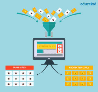
Naive Bayes classifiers are a popular statistical technique of e-mail filtering. They typically use a bag of words features to identify spam e-mail, an approach commonly used in text classification. Naive Bayes classifiers work by correlating the use of tokens (typically words, or sometimes other things), with a spam and non-spam e-mails and then using Bayes’ theorem to calculate a probability that an email is or is not spam.

Particular words have particular probabilities of occurring in spam email and in legitimate email. For instance, most email users will frequently encounter the word “Lottery” and “Luck Draw” in spam email, but will seldom see it in other emails. Each word in the email contributes to the email’s spam probability or only the most interesting words. This contribution is called the posterior probability and is computed using Bayes’ theorem. Then, the email’s spam probability is computed over all words in the email, and if the total exceeds a certain threshold (say 95%), the filter will mark the email as a spam.

Medical Diagnosis:

Nowadays modern hospitals are well equipped with monitoring and other data collection devices resulting in enormous data which are collected continuously through health examination and medical treatment. One of the main advantages of the Naive Bayes approach which is appealing to physicians is that “all the available information is used to explain the decision”. This explanation seems to be “natural” for medical diagnosis and prognosis i.e. is close to the way how physicians diagnose patients.

When dealing with medical data, Naïve Bayes classifier takes into account evidence from many attributes to make the final prediction and provides transparent explanations of its decisions and therefore it is considered as one of the most useful classifiers to support physicians’ decisions.

Weather Prediction:

Weather is one of the most influential factors in our daily life, to an extent that it may affect the economy of a country that depends on occupation like agriculture.  Weather prediction has been a challenging problem in the meteorological department for years. Even after the technological and scientific advancement, the accuracy in prediction of weather has never been sufficient.

A Bayesian approach based model for weather prediction is used, where posterior probabilities are used to calculate the likelihood of each class label for input data instance and the one with maximum likelihood is considered resulting output.

Step By Step Implementation of Naive Bayes

Here we have a dataset comprising of 768 Observations of women aged 21 and older. The dataset describes instantaneous measurement taken from patients, like age, blood workup, the number of times pregnant. Each record has a class value that indicates whether the patient suffered an onset of diabetes within 5 years. The values are 1 for Diabetic and 0 for Non-Diabetic.

Now, Let’s continue our Naive Bayes Blog and understand all the steps one by one. I,ve broken the whole process down into the following steps:

• Handle Data
• Summarize Data
• Make Predictions
• Evaluate Accuracy

Step 1: Handle Data

The first thing we need to do is load our data file. The data is in CSV format without a header line or any quotes. We can open the file with the open function and read the data lines using the reader function in the CSV module.

import csv
import math
import random


def loadCsv(filename):
lines = csv.reader(open(r'C:UsersKislayDesktoppima-indians-diabetes.data.csv'))
dataset = list(lines)
for i in range(len(dataset)):
dataset[i] = [float(x) for x in dataset[i]]
return dataset

Now we need to split the data into training and testing dataset.

def splitDataset(dataset, splitRatio):
trainSize = int(len(dataset) * splitRatio)
trainSet = []
copy = list(dataset)
while len(trainSet) < trainSize:
index = random.randrange(len(copy))
trainSet.append(copy.pop(index))
return [trainSet, copy]

Step 2: Summarize the Data

The summary of the training data collected involves the mean and the standard deviation for each attribute, by class value. These are required when making predictions to calculate the probability of specific attribute values belonging to each class value.

We can break the preparation of this summary data down into the following sub-tasks:

• Separate Data By Class

def separateByClass(dataset):
separated = {}
for i in range(len(dataset)):
vector = dataset[i]
if (vector[-1] not in separated):
separated[vector[-1]] = []
separated[vector[-1]].append(vector)
return separated

• Calculate Mean

def mean(numbers):
return sum(numbers)/float(len(numbers))

• Calculate Standard Deviation

def stdev(numbers):
avg = mean(numbers)
variance = sum([pow(x-avg,2) for x in numbers])/float(len(numbers)-1)
return math.sqrt(variance)

• Summarize Dataset

def summarize(dataset):
summaries = [(mean(attribute), stdev(attribute)) for attribute in zip(*dataset)]
del summaries[-1]
return summaries

• Summarize Attributes By Class

def summarizeByClass(dataset):
separated = separateByClass(dataset)
summaries = {}
for classValue, instances in separated.items():
summaries[classValue] = summarize(instances)
return summaries

Step 3: Making Predictions

We are now ready to make predictions using the summaries prepared from our training data. Making predictions involves calculating the probability that a given data instance belongs to each class, then selecting the class with the largest probability as the prediction. We need to perform the following tasks:

• Calculate Gaussian Probability Density Function

def calculateProbability(x, mean, stdev):
exponent = math.exp(-(math.pow(x-mean,2)/(2*math.pow(stdev,2))))
return (1/(math.sqrt(2*math.pi)*stdev))*exponent

• Calculate Class Probabilities

def calculateClassProbabilities(summaries, inputVector):
probabilities = {}
for classValue, classSummaries in summaries.items():
probabilities[classValue] = 1
for i in range(len(classSummaries)):
mean, stdev = classSummaries[i]
x = inputVector[i]
probabilities[classValue] *= calculateProbability(x, mean, stdev)
return probabilities

• Make a Prediction

def predict(summaries, inputVector):
probabilities = calculateClassProbabilities(summaries, inputVector)
bestLabel, bestProb = None, -1
for classValue, probability in probabilities.items():
if bestLabel is None or probability > bestProb:
bestProb = probability
bestLabel = classValue
return bestLabel

• Make Predictions

def getPredictions(summaries, testSet):
predictions = []
for i in range(len(testSet)):
result = predict(summaries, testSet[i])
predictions.append(result)
return predictions

• Get Accuracy

def getAccuracy(testSet, predictions):
correct = 0
for x in range(len(testSet)):
if testSet[x][-1] == predictions[x]:
correct += 1
return (correct/float(len(testSet)))*100.0

Finally, we define our main function where we call all these methods we have defined, one by one to get the accuracy of the model we have created.

def main():
filename = 'pima-indians-diabetes.data.csv'
splitRatio = 0.67
dataset = loadCsv(filename)
trainingSet, testSet = splitDataset(dataset, splitRatio)
print('Split {0} rows into train = {1} and test = {2} rows'.format(len(dataset),len(trainingSet),len(testSet)))
#prepare model
summaries = summarizeByClass(trainingSet)
#test model
predictions = getPredictions(summaries, testSet)
accuracy = getAccuracy(testSet, predictions)
print('Accuracy: {0}%'.format(accuracy))

main()

Output:

So here as you can see the accuracy of our Model is 66 %.  Now, This value differs from model to model and also the split ratio.

Now that we have seen the steps involved in the Naive Bayes Classifier, Python comes with a library SKLEARN  which makes all the above-mentioned steps easy to implement and use. Let’s continue our Naive Bayes Tutorial and see how this can be implemented.

Naive Bayes with SKLEARN

For our research, we are going to use the IRIS dataset, which comes with the sklearn library. The dataset contains 3 classes of 50 instances each, where each class refers to a type of iris plant. Here we are going to use the GaussianNB model, which is already available in the SKLEARN Library.

Importing Libraries and Loading Datasets

from sklearn import datasets
from sklearn import metrics
from sklearn.naive_bayes import GaussianNB

 

dataset = datasets.load_iris()

Creating our Naive Bayes Model using Sklearn

Here we have a GaussianNB() method that performs exactly the same functions as the code explained above

model = GaussianNB()
model.fit(dataset.data, dataset.target)

Making Predictions

expected = dataset.target
predicted = model.predict(dataset.data)

Getting Accuracy and Statistics

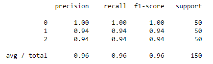
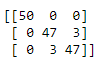
Here we will create a classification report that contains the various statistics required to judge a model. After that, we will create a confusion matrix which will give us a clear idea of the Accuracy and the fitting of the model.

print(metrics.classification_report(expected, predicted))
print(metrics.confusion_matrix(expected, predicted))

Classification Report:

Confusion Matrix:

As you can see all the hundreds of lines of code can be summarized into just a few lines of code with this powerful library.

So, with this, we come to the end of this Naive Bayes Tutorial Blog. I hope you enjoyed this blog. If you are reading this, Congratulations! You are no longer a newbie to Naive Bayes. Try out this simple example on your systems now.

Now that you have understood the basics of Naive Bayes, check out the Python Certification Training for Data Science by Edureka, a trusted online learning company with a network of more than 250,000 satisfied learners spread across the globe. Edureka’s Python course helps you gain expertise in Quantitative Analysis, data mining, and the presentation of data to see beyond the numbers by transforming your career into Data Scientist role. You will use libraries like Pandas, Numpy, Matplotlib, Scikit and master the concepts like Python Machine Learning Algorithms such as Regression, Clustering, Decision Trees, Random Forest, Naïve Bayes and Q-Learning and Time Series. Throughout the Course, you’ll be solving real-life case studies on Media, Healthcare, Social Media, Aviation, HR and so on

Got a question for us? Please mention it in the comments section and we will get back to you.