
Data Science with Python Certification Course
- 132k Enrolled Learners
- Weekend
- Live Class
(49300)


 Copy Link!
Machine Learning has become the most in-demand skill in the market. It is essential to know the various Machine Learning Algorithms and how they work. In this blog on Naive Bayes In R, I intend to help you learn about how Naive Bayes works and how it can be implemented using the R language.
To get in-depth knowledge on Data Science, you can enroll for live Data Science Certification Training by Edureka with 24/7 support and lifetime access.
The following topics are covered in this blog:
Naive Bayes is a Supervised Machine Learning algorithm based on the Bayes Theorem that is used to solve classification problems by following a probabilistic approach. It is based on the idea that the predictor variables in a Machine Learning model are independent of each other. Meaning that the outcome of a model depends on a set of independent variables that have nothing to do with each other.
In real-world problems, predictor variables aren’t always independent of each other, there are always some correlations between them. Since Naive Bayes considers each predictor variable to be independent of any other variable in the model, it is called ‘Naive’.
Now let’s understand the logic behind the Naive Bayes algorithm.
The principle behind Naive Bayes is the Bayes theorem also known as the Bayes Rule. The Bayes theorem is used to calculate the conditional probability, which is nothing but the probability of an event occurring based on information about the events in the past. Mathematically, the Bayes theorem is represented as:

Bayes Theorem – Naive Bayes In R – Edureka
In the above equation:
Formally, the terminologies of the Bayesian Theorem are as follows:
Therefore, the Bayes theorem can be summed up as:
Posterior=(Likelihood).(Proposition prior probability)/Evidence prior probability
It can also be considered in the following manner:
Given a Hypothesis H and evidence E, Bayes Theorem states that the relationship between the probability of Hypothesis before getting the evidence P(H) and the probability of the hypothesis after getting the evidence P(H|E) is:
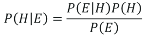
Bayes Theorem In Terms Of Hypothesis – Naive Bayes In R – Edureka
Now that you know what the Bayes Theorem is, let’s see how it can be derived.
The main aim of the Bayes Theorem is to calculate the conditional probability. The Bayes Rule can be derived from the following two equations:
The below equation represents the conditional probability of A, given B:
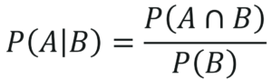
Deriving Bayes Theorem Equation 1 – Naive Bayes In R – Edureka
The below equation represents the conditional probability of B, given A:
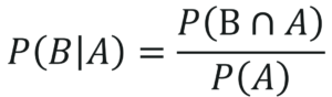
Deriving Bayes Theorem Equation 2 – Naive Bayes In R – Edureka
Therefore, on combining the above two equations we get the Bayes Theorem:

Bayes Theorem – Naive Bayes In R – Edureka
The above equation was for a single predictor variable, however, in real-world applications, there are more than one predictor variables and for a classification problem, there is more than one output class. The classes can be represented as, C1, C2,…, Ck and the predictor variables can be represented as a vector, x1,x2,…,xn.
The objective of a Naive Bayes algorithm is to measure the conditional probability of an event with a feature vector x1,x2,…,xn belonging to a particular class Ci,

On computing the above equation, we get:
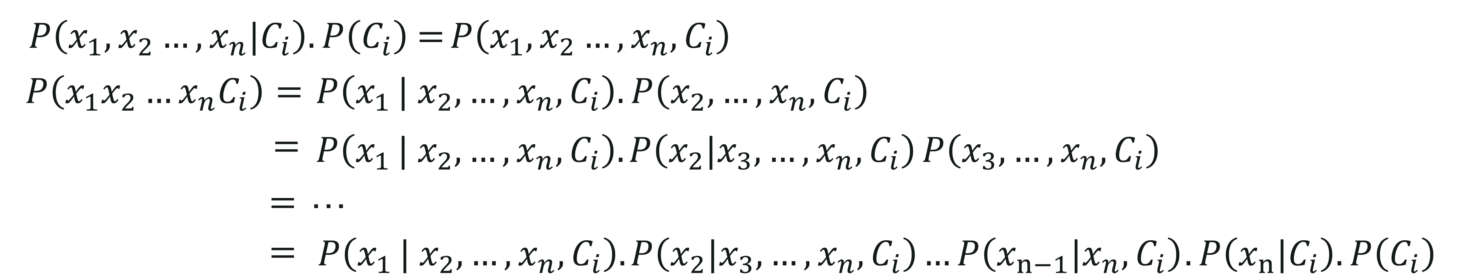
However, the conditional probability, i.e., P(xj|xj+1,…,xn,Ci) sums down to P(xj|Ci) since each predictor variable is independent in Naive Bayes.
The final equation comes down to:
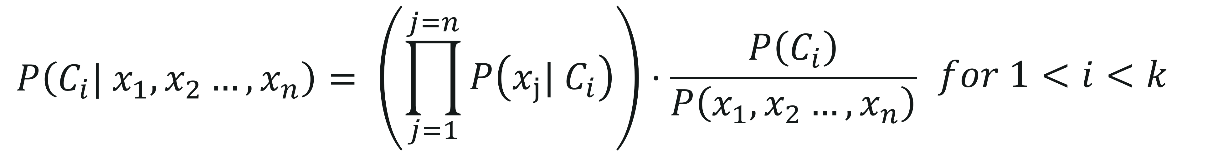
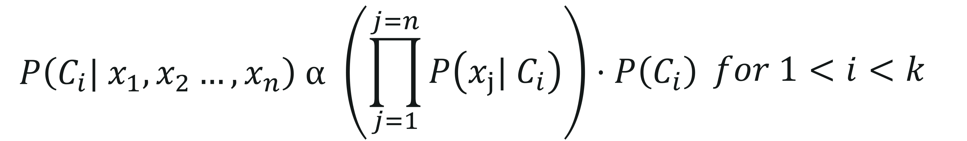
Here, P(x1,x2,…,xn) is constant for all the classes, therefore we get:
To get a better understanding of how Naive Bayes works, let’s look at an example.
Consider a data set with 1500 observations and the following output classes:
The Predictor variables are categorical in nature i.e., they store two values, either True or False:
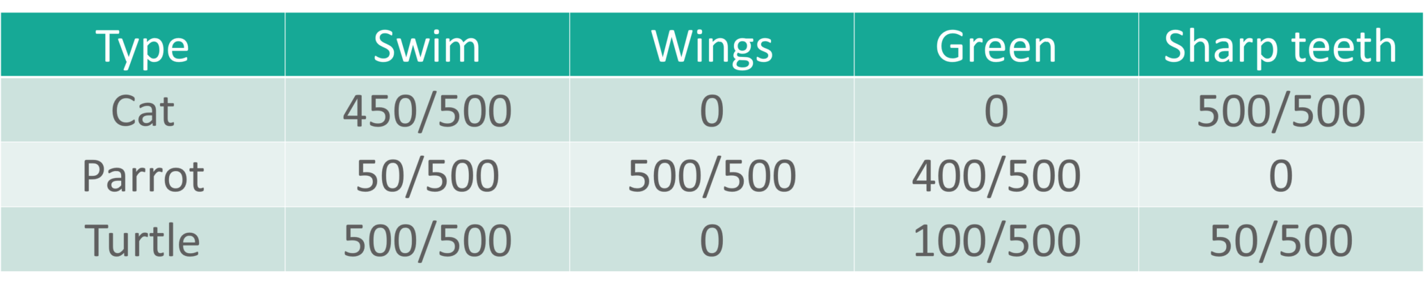
Naive Bayes Example – Naive Bayes In R – Edureka
From the above table, we can summarise that:
The class of type cats shows that:
The class of type Parrot shows that:
The class of type Turtle shows:
Now, with the available data, let’s classify the following observation into one of the output classes (Cats, Parrot or Turtle) by using the Naive Bayes Classifier.

The goal here is to predict whether the animal is a Cat, Parrot or a Turtle based on the defined predictor variables (swim, wings, green, sharp teeth).
To solve this, we will use the Naive Bayes approach,
P(H|Multiple Evidences) = P(C1| H)* P(C2|H) ……*P(Cn|H) * P(H) / P(Multiple Evidences)
In the observation, the variables Swim and Green are true and the outcome can be any one of the animals (Cat, Parrot, Turtle).
To check if the animal is a cat:
P(Cat | Swim, Green) = P(Swim|Cat) * P(Green|Cat) * P(Cat) / P(Swim, Green)
= 0.9 * 0 * 0.333 / P(Swim, Green)
= 0
To check if the animal is a Parrot:
P(Parrot| Swim, Green) = P(Swim|Parrot) * P(Green|Parrot) * P(Parrot) / P(Swim, Green)
= 0.1 * 0.80 * 0.333 / P(Swim, Green)
= 0.0264/ P(Swim, Green)
To check if the animal is a Turtle:
P(Turtle| Swim, Green) = P(Swim|Turtle) * P(Green|Turtle) * P(Turtle) / P(Swim, Green)
= 1 * 0.2 * 0.333 / P(Swim, Green)
= 0.0666/ P(Swim, Green)
For all the above calculations the denominator is the same i.e, P(Swim, Green). The value of P(Turtle| Swim, Green) is greater than P(Parrot| Swim, Green), therefore we can correctly predict the class of the animal as Turtle.
Now let’s see how you can implement Naive Bayes using the R language.
Problem Statement: To study a Diabetes data set and build a Machine Learning model that predicts whether or not a person has Diabetes.
Data Set Description: The given data set contains 100s of observations of patients along with their health details. Here’s a list of the predictor variables that will help us classify a patient as either Diabetic or Normal:
The response variable or the output variable is:
Logic: To build a Naive Bayes model in order to classify patients as either Diabetic or normal by studying their medical records such as Glucose level, age, BMI, etc.
Now that you know the objective of this demo, let’s get our brains working and start coding. For this demo, I’ll be using the R language in order to build the model.
If you wish to learn more about R programming, you can go through this video recorded by our R Programming Experts.
Now, let’s begin.
Step 1: Install and load the requires packages
#Loading required packages
install.packages('tidyverse')
library(tidyverse)
install.packages('ggplot2')
library(ggplot2)
install.packages('caret')
library(caret)
install.packages('caretEnsemble')
library(caretEnsemble)
install.packages('psych')
library(psych)
install.packages('Amelia')
library(Amelia)
install.packages('mice')
library(mice)
install.packages('GGally')
library(GGally)
install.packages('rpart')
library(rpart)
install.packages('randomForest')
library(randomForest)
Step 2: Import the data set
#Reading data into R
data<- read.csv("/Users/Zulaikha_Geer/Desktop/NaiveBayesData/diabetes.csv")
Before we study the data set let’s convert the output variable (‘Outcome’) into a categorical variable. This is necessary because our output will be in the form of 2 classes, True or False. Where true will denote that a patient has diabetes and false denotes that a person is diabetes free.
#Setting outcome variables as categorical
data$Outcome <- factor(data$Outcome, levels = c(0,1), labels = c("False", "True"))
Step 3: Studying the Data Set
#Studying the structure of the data

str(data)
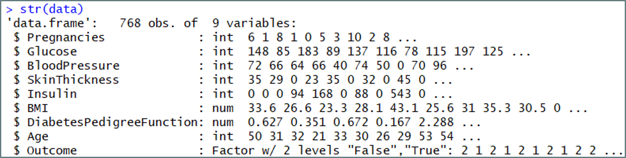
Understanding the data set – Naive Bayes In R – Edureka
head(data)
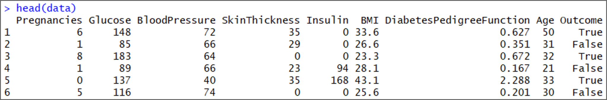
Understanding the data set – Naive Bayes In R – Edureka
describe(data)
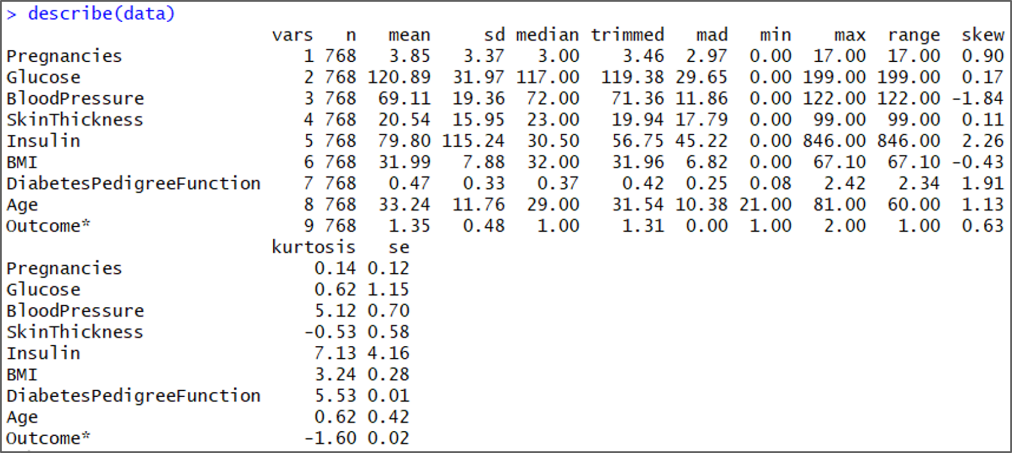
Understanding the data set – Naive Bayes In R – Edureka
Step 4: Data Cleaning
While analyzing the structure of the data set, we can see that the minimum values for Glucose, Bloodpressure, Skinthickness, Insulin, and BMI are all zero. This is not ideal since no one can have a value of zero for Glucose, blood pressure, etc. Therefore, such values are treated as missing observations.
In the below code snippet, we’re setting the zero values to NA’s:
#Convert '0' values into NA
data[, 2:7][data[, 2:7] == 0] <- NA
To check how many missing values we have now, let’s visualize the data:
#visualize the missing data
missmap(data)
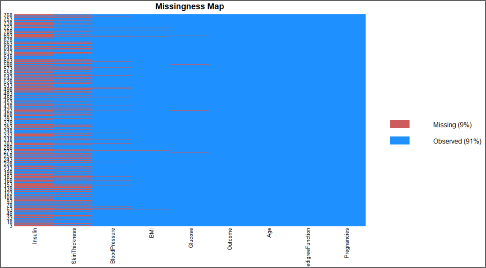
Missing Data Plot – Naive Bayes In R – Edureka
The above illustrations show that our data set has plenty missing values and removing all of them will leave us with an even smaller data set, therefore, we can perform imputations by using the mice package in R.
#Use mice package to predict missing values
mice_mod <- mice(data[, c("Glucose","BloodPressure","SkinThickness","Insulin","BMI")], method='rf')
mice_complete <- complete(mice_mod)

iter imp variable
1 1 Glucose BloodPressure SkinThickness Insulin BMI
1 2 Glucose BloodPressure SkinThickness Insulin BMI
1 3 Glucose BloodPressure SkinThickness Insulin BMI
1 4 Glucose BloodPressure SkinThickness Insulin BMI
1 5 Glucose BloodPressure SkinThickness Insulin BMI
2 1 Glucose BloodPressure SkinThickness Insulin BMI
2 2 Glucose BloodPressure SkinThickness Insulin BMI
2 3 Glucose BloodPressure SkinThickness Insulin BMI
2 4 Glucose BloodPressure SkinThickness Insulin BMI
2 5 Glucose BloodPressure SkinThickness Insulin BMI

#Transfer the predicted missing values into the main data set
data$Glucose <- mice_complete$Glucose
data$BloodPressure <- mice_complete$BloodPressure
data$SkinThickness <- mice_complete$SkinThickness
data$Insulin<- mice_complete$Insulin
data$BMI <- mice_complete$BMI
To check if there are still any missing values, let’s use the missmap plot:
missmap(data)
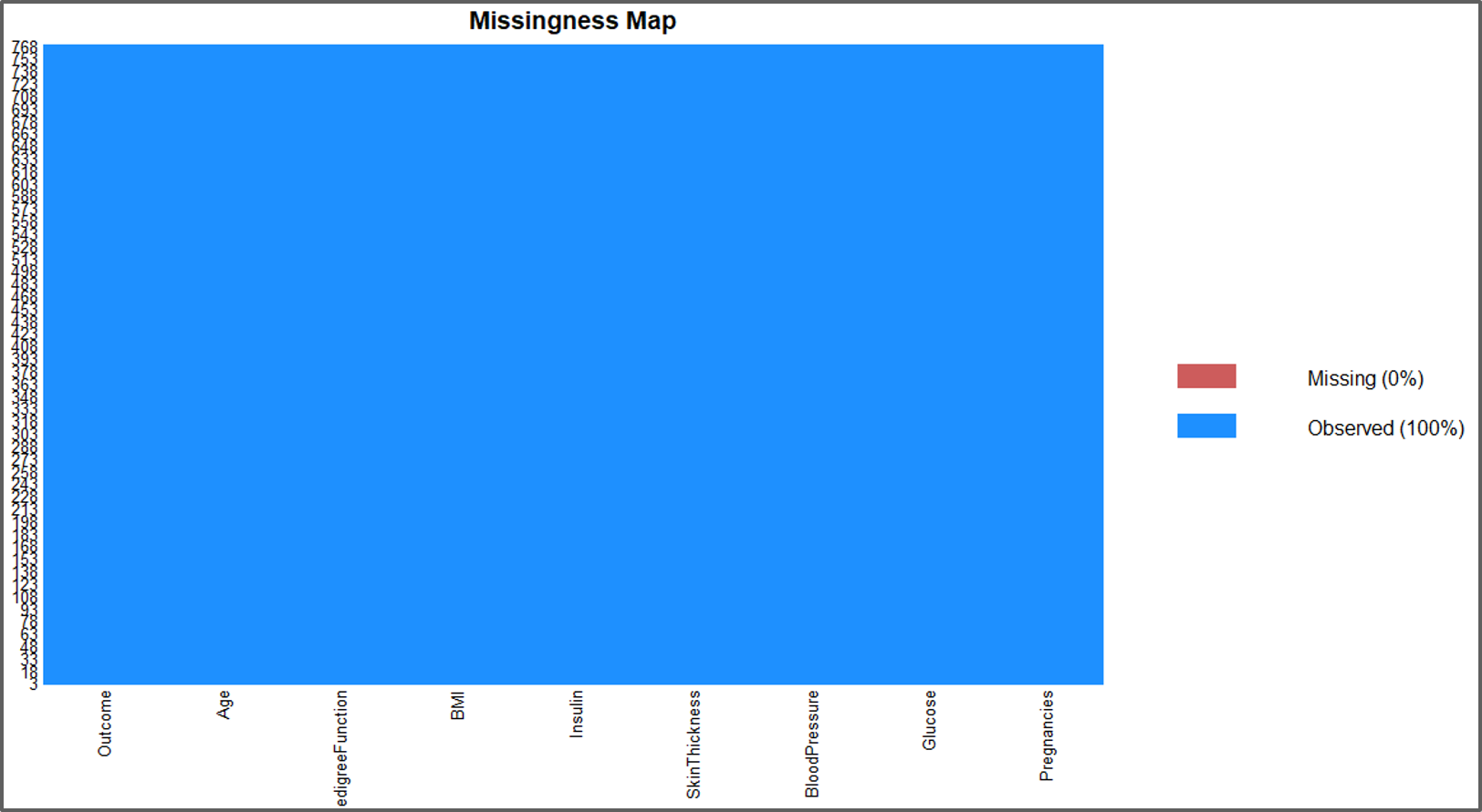
Using Mice Package In R – Naive Bayes In R – Edureka
The output looks good, there is no missing data.
Step 5: Exploratory Data Analysis
Now let’s perform a couple of visualizations to take a better look at each variable, this stage is essential to understand the significance of each predictor variable.
#Data Visualization
#Visual 1
ggplot(data, aes(Age, colour = Outcome)) +
geom_freqpoly(binwidth = 1) + labs(title="Age Distribution by Outcome")
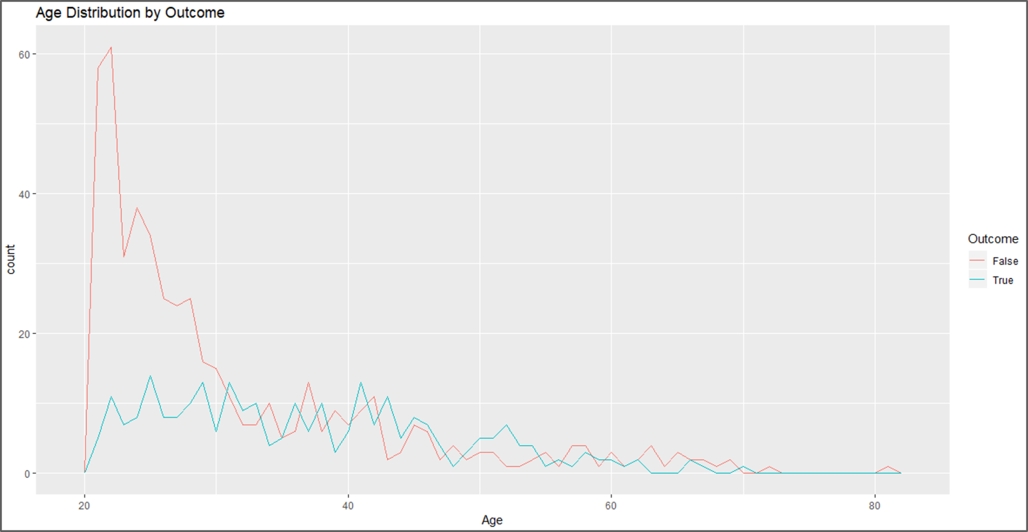
Data Visualization – Naive Bayes In R – Edureka
#visual 2
c <- ggplot(data, aes(x=Pregnancies, fill=Outcome, color=Outcome)) +
geom_histogram(binwidth = 1) + labs(title="Pregnancy Distribution by Outcome")
c + theme_bw()
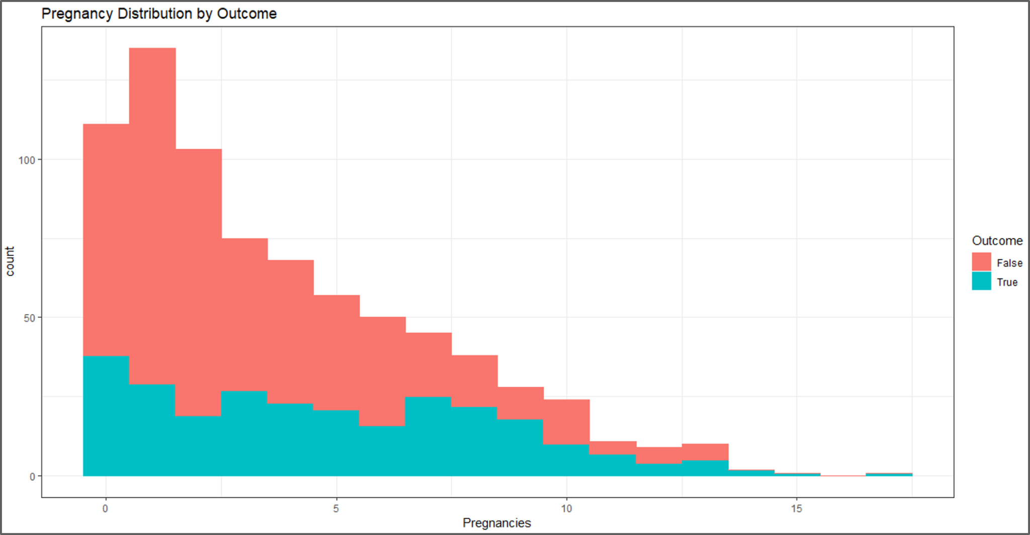
Data Visualization – Naive Bayes In R – Edureka
#visual 3
P <- ggplot(data, aes(x=BMI, fill=Outcome, color=Outcome)) +
geom_histogram(binwidth = 1) + labs(title="BMI Distribution by Outcome")
P + theme_bw()
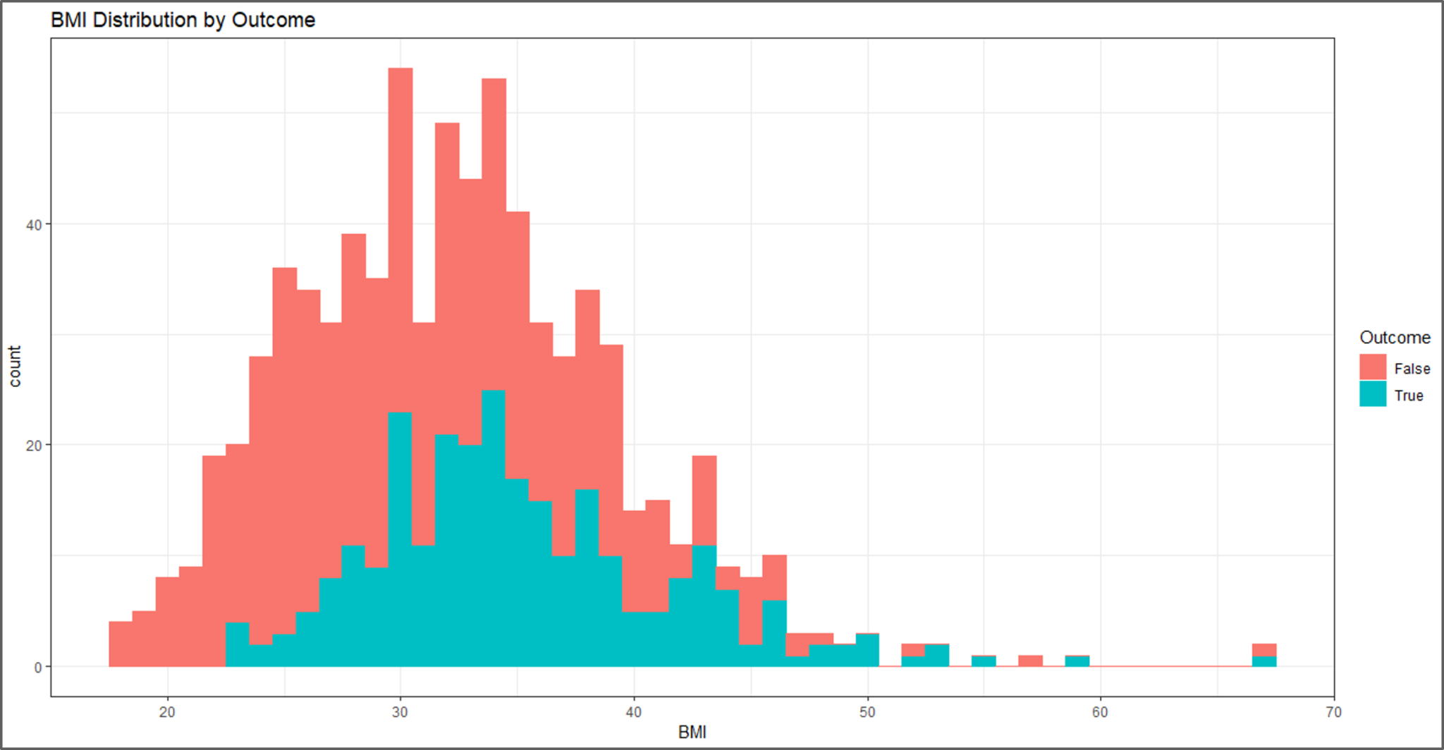
Data Visualization – Naive Bayes In R – Edureka
#visual 4
ggplot(data, aes(Glucose, colour = Outcome)) +
geom_freqpoly(binwidth = 1) + labs(title="Glucose Distribution by Outcome")
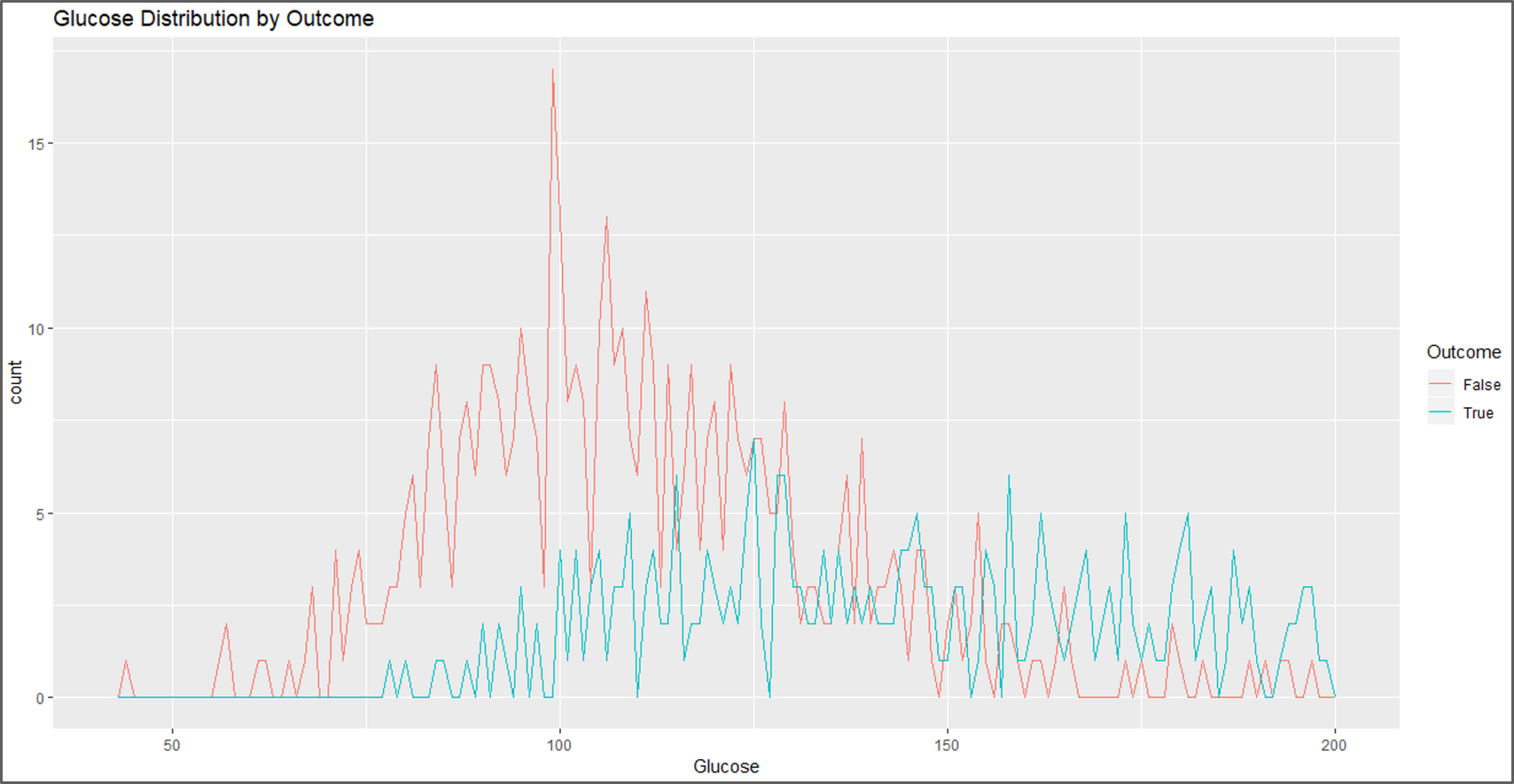
Data Visualization – Naive Bayes In R – Edureka
#visual 5
ggpairs(data)
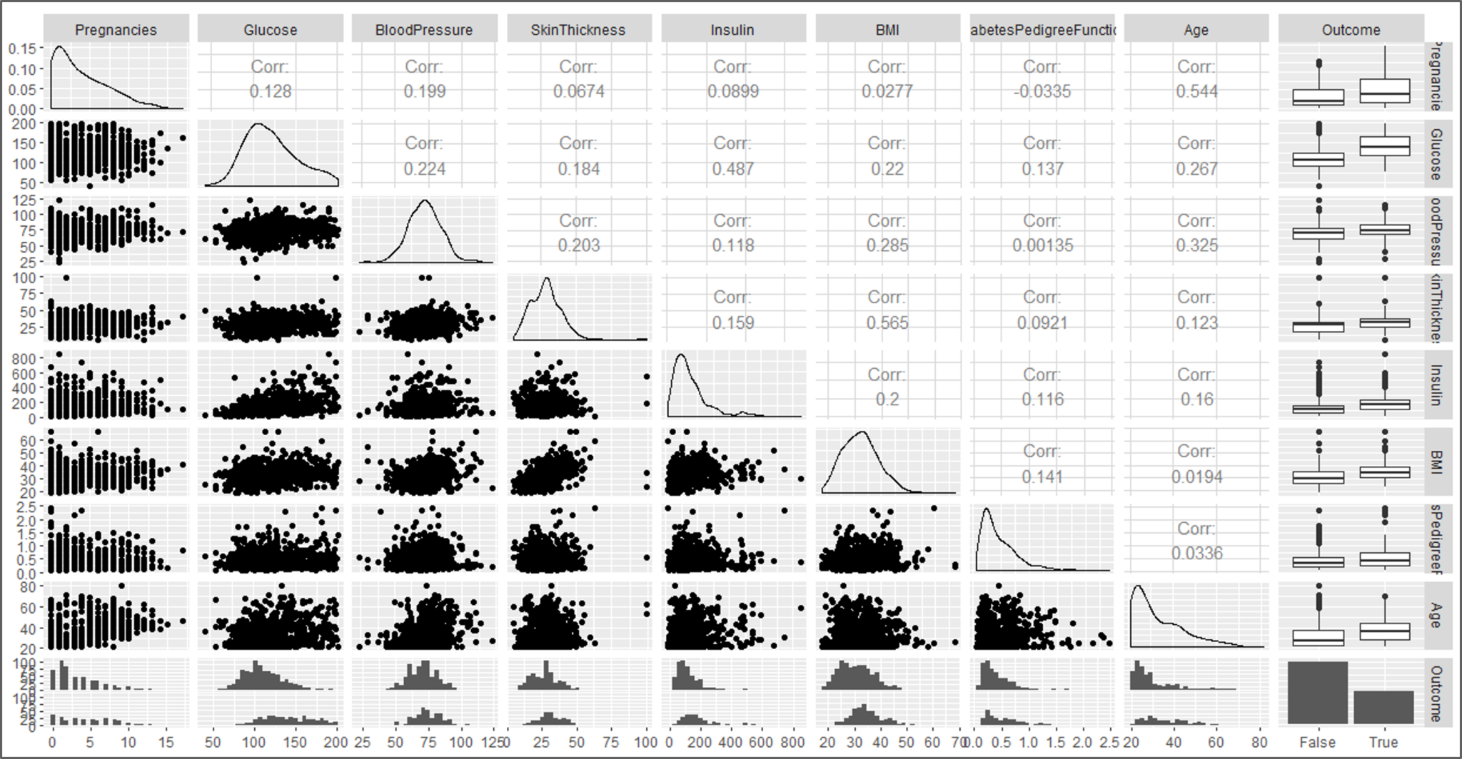
Data Visualization – Naive Bayes In R – Edureka
Step 6: Data Modelling
This stage begins with a process called Data Splicing, wherein the data set is split into two parts:
#Building a model
#split data into training and test data sets
indxTrain <- createDataPartition(y = data$Outcome,p = 0.75,list = FALSE)
training <- data[indxTrain,]
testing <- data[-indxTrain,] #Check dimensions of the split > prop.table(table(data$Outcome)) * 100

False True
65.10417 34.89583

> prop.table(table(training$Outcome)) * 100

False True
65.10417 34.89583

> prop.table(table(testing$Outcome)) * 100

False True
65.10417 34.89583
For comparing the outcome of the training and testing phase let’s create separate variables that store the value of the response variable:
#create objects x which holds the predictor variables and y which holds the response variables
x = training[,-9]
y = training$Outcome
Now it’s time to load the e1071 package that holds the Naive Bayes function. This is an in-built function provided by R.
library(e1071)
After loading the package, the below code snippet will create Naive Bayes model by using the training data set:
model = train(x,y,'nb',trControl=trainControl(method='cv',number=10))

> model
Naive Bayes

576 samples
8 predictor
2 classes: 'False', 'True'

No pre-processing
Resampling: Cross-Validated (10 fold)
Summary of sample sizes: 518, 518, 519, 518, 519, 518, ...
Resampling results across tuning parameters:

usekernel Accuracy Kappa
FALSE 0.7413793 0.4224519
TRUE 0.7622505 0.4749285

Tuning parameter 'fL' was held constant at a value of 0
Tuning parameter 'adjust' was held
constant at a value of 1
Accuracy was used to select the optimal model using the largest value.
The final values used for the model were fL = 0, usekernel = TRUE and adjust = 1.
We thus created a predictive model by using the Naive Bayes Classifier.
Step 7: Model Evaluation
To check the efficiency of the model, we are now going to run the testing data set on the model, after which we will evaluate the accuracy of the model by using a Confusion matrix.
#Model Evaluation
#Predict testing set
Predict <- predict(model,newdata = testing ) #Get the confusion matrix to see accuracy value and other parameter values > confusionMatrix(Predict, testing$Outcome )
Confusion Matrix and Statistics

Reference
Prediction False True
False 91 18
True 34 49

Accuracy : 0.7292
95% CI : (0.6605, 0.7906)
No Information Rate : 0.651
P-Value [Acc > NIR] : 0.01287

Kappa : 0.4352

Mcnemar's Test P-Value : 0.03751

Sensitivity : 0.7280
Specificity : 0.7313
Pos Pred Value : 0.8349
Neg Pred Value : 0.5904
Prevalence : 0.6510
Detection Rate : 0.4740
Detection Prevalence : 0.5677
Balanced Accuracy : 0.7297

'Positive' Class : False
The final output shows that we built a Naive Bayes classifier that can predict whether a person is diabetic or not, with an accuracy of approximately 73%.
To summaries the demo, let’s draw a plot that shows how each predictor variable is independently responsible for predicting the outcome.
#Plot Variable performance
X <- varImp(model)
plot(X)
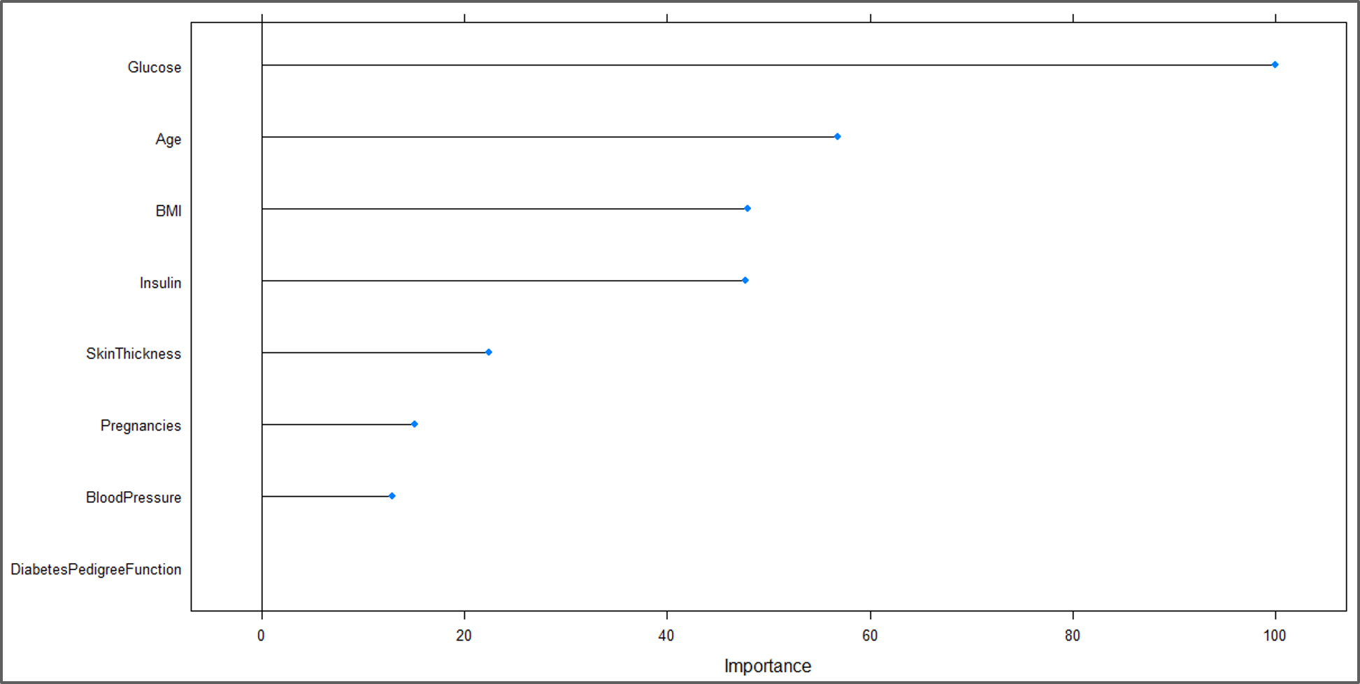
Variable Performance Plot – Naive Bayes In R – Edureka
From the above illustration, it is clear that ‘Glucose’ is the most significant variable for predicting the outcome.
Now that you know how Naive Bayes works, I’m sure you’re curious to learn more about the various Machine learning algorithms. Here’s a list of blogs on Machine Learning Algorithms, do give them a read:
So, with this, we come to the end of this blog. I hope you all found this blog informative. If you have any thoughts to share, please comment them below. Stay tuned for more blogs like these!
If you are looking for online structured training in Data Science, edureka! has a specially curated Data Science course which helps you gain expertise in Statistics, Data Wrangling, Exploratory Data Analysis, Machine Learning Algorithms like K-Means Clustering, Decision Trees, Random Forest, Naive Bayes. You’ll learn the concepts of Time Series, Text Mining and an introduction to Deep Learning as well. New batches for this course are starting soon!!


 Thank you for registering Join Edureka Meetup community for 100+ Free Webinars each month JOIN MEETUP GROUP