A Complete Guide To Math And Statistics For Data Science

Introduction

As Josh Wills once said,

Math and Statistics for Data Science are essential because these disciples form the basic foundation of all the Machine Learning Algorithms. In fact, Mathematics is behind everything around us, from shapes, patterns and colors, to the count of petals in a flower. Mathematics is embedded in each and every aspect of our lives.

Although having a good understanding of programming languages, Machine Learning algorithms and following a data-driven approach is necessary to become a Data Scientist, Data Science isn’t all about these fields. In this blog post, you will understand the importance of Math and Statistics for Data Science and how they can be used to build Machine Learning models.

To get in-depth knowledge on Data Science and the various Machine Learning Algorithms, you can enroll for live Data Science with Python  Course by Edureka with 24/7 support and lifetime access.

Introduction To Statistics

To become a successful Data Scientist you must know your basics. Math and Stats are the building blocks of Machine Learning algorithms. It is important to know the techniques behind various Machine Learning algorithms in order to know how and when to use them. Now the question arises, what exactly is Statistics?

Statistics – Math And Statistics For Data Science – Edureka

Statistics is used to process complex problems in the real world so that Data Scientists and Analysts can look for meaningful trends and changes in Data. In simple words, Statistics can be used to derive meaningful insights from data by performing mathematical computations on it.

Several Statistical functions, principles and algorithms are implemented to analyse raw data, build a Statistical Model and infer or predict the result.

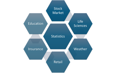
Statistics Applications – Math And Statistics For Data Science – Edureka

The field of Statistics has an influence over all domains of life, the Stock market, life sciences, weather, retail, insurance and education are but to name a few.

Moving ahead. let’s discuss the basic terminologies in Statistics.

Terminologies In Statistics – Statistics For Data Science

One should be aware of a few key statistical terminologies while dealing with Statistics for Data Science. I’ve discussed these terminologies below:

• Population is the set of sources from which data has to be collected.
• A Sample is a subset of the Population
• A Variable is any characteristics, number, or quantity that can be measured or counted. A variable may also be called a data item.
• Also known as a statistical model, A statistical Parameter or population parameter is a quantity that indexes a family of probability distributions. For example, the mean, median, etc of a population.

Before we move any further and discuss the categories of Statistics, let’s look at the types of analysis.

Types Of Analysis

An analysis of any event can be done in one of two ways:

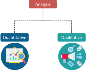
Types Of Analysis – Math And Statistics For Data Science – Edureka

1. Quantitative Analysis: Quantitative Analysis or the Statistical Analysis is the science of collecting and interpreting data with numbers and graphs to identify patterns and trends.
2. Qualitative Analysis: Qualitative or Non-Statistical Analysis gives generic information and uses text, sound and other forms of media to do so.

For example, if I want a purchase a coffee from Starbucks, it is available in Short, Tall and Grande. This is an example of Qualitative Analysis. But if a store sells 70 regular coffees a week, it is Quantitative Analysis because we have a number representing the coffees sold per week.

Although the purpose of both these analyses is to provide results, Quantitative analysis provides a clearer picture hence making it crucial in analytics.

Categories In Statistics

There are two main categories in Statistics, namely:

1. Descriptive Statistics
2. Inferential Statistics

Descriptive Statistics

Descriptive Statistics helps organize data and focuses on the characteristics of data providing parameters.

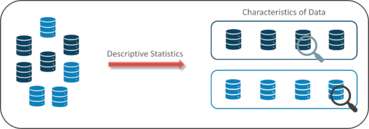
Descriptive Statistics – Math And Statistics For Data Science – Edureka

Suppose you want to study the average height of students in a classroom, in descriptive statistics you would record the heights of all students in the class and then you would find out the maximum, minimum and average height of the class.

Descriptive Statistics Example – Math And Statistics For Data Science – Edureka

Inferential Statistics

Inferential statistics generalizes a large data set and applies probability to arrive at a conclusion. It allows you to infer parameters of the population based on sample stats and build models on it.

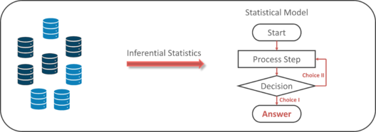
Inferential Statistics – Math And Statistics For Data Science – Edureka

So, if we consider the same example of finding the average height of students in a class, in Inferential Statistics, you will take a sample set of the class, which is basically a few people from the entire class. You already have had grouped the class into tall, average and short. In this method, you basically build a statistical model and expand it for the entire population in the class.

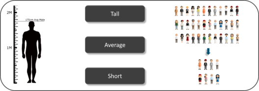
Inferential Statistics Example – Math And Statistics For Data Science – Edureka

Now let’s focus our attention on Descriptive Statistics and see how it can be used to solve analytical problems.

Understanding Descriptive Analysis

When we try to represent data in the form of graphs, like histograms, line plots, etc. the data is represented based on some kind of central tendency. Central tendency measures like, mean, median, or measures of the spread, etc are used for statistical analysis. To better understand Statistics lets discuss the different measures in Statistics with the help of an example.

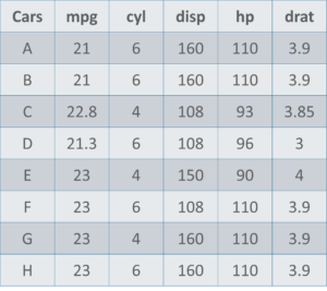
Cars Data Set – Math And Statistics For Data Science – Edureka

Here is a sample data set of cars containing the variables:

1. Cars
2. Mileage per Gallon (mpg)
3. Cylinder Type (cyl)
4. Displacement (disp)
5. Horse Power (hp)
6. Real Axle Ratio (drat).

Before we move any further, let’s define the main Measures of the Center or Measures of Central tendency.

Measures Of The Center

1. Mean: Measure of average of all the values in a sample is called Mean.
2. Median: Measure of the central value of the sample set is called Median.
   
3. Mode: The value most recurrent in the sample set is known as Mode.
   

Using descriptive Analysis, you can analyse each of the variables in the sample data set for mean, standard deviation, minimum and maximum.

• If we want to find out the mean or average horsepower of the cars among the population of cars, we will check and calculate the average of all values. In this case, we’ll take the sum of the Horse Power of each car, divided by the total number of cars:

Mean = (110+110+93+96+90+110+110+110)/8 = 103.625

• If we want to find out the center value of mpg among the population of cars, we will arrange the mpg values in ascending or descending order and choose the middle value. In this case, we have 8 values which is an even entry. Hence we must take the average of the two middle values.

The mpg for 8 cars: 21,21,21.3,22.8,23,23,23,23
Median = (22.8+23 )/2 = 22.9

• If we want to find out the most common type of cylinder among the population of cars, we will check the value which is repeated most number of times. Here we can see that the cylinders come in two values, 4 and 6. Take a look at the data set, you can see that the most recurring value is 6. Hence 6 is our Mode.

Measures Of The Spread

Just like the measure of center, we also have measures of the spread, which comprises of the following measures:

1. Range: It is the given measure of how spread apart the values in a data set are.
2. Inter Quartile Range (IQR): It is the measure of variability, based on dividing a data set into quartiles.
3. Variance: It describes how much a random variable differs from its expected value. It entails computing squares of deviations.
   1. Deviation is the difference between each element from the mean.
   2. Population Variance is the average of squared deviations
   3. Sample Variance is the average of squared differences from the mean
4. Standard Deviation: It is the measure of the dispersion of a set of data from its mean.

Now that we’ve seen the stats and math behind Descriptive analysis, let’s try to work it out in R.

If you want to learn more about the R language, you can check out this video recorded by our R programming specialists.

Statistics In R

There are n number of reasons why the world is moving to R. A couple of them are enlisted below:

• R is open-source and freely available. Unlike SAS or Matlab, you can freely install, use, update, clone, modify, redistribute and resell R.
• R is cross-platform compatible. It is compatible to run on Windows, Mac OS X and Linux. It can also import data from Microsoft Excel, Microsoft Access, MySQL, SQLite, Oracle and other programs.
• R is a powerful scripting language and it can handle large, complex data sets.
• R is highly flexible and evolved. Many new developments in statistics first appear as R packages.

If you’re still not convinced about why you must use R, the Statistical language, give this R Tutorial blog a read.

Now let’s move ahead and implement Descriptive Statistics in R.

Descriptive Statistics In R

It’s always best to perform practical implementation to better understand a concept. In this section, we’ll be executing a small demo that will show you how to calculate the Mean, Median, Mode, Variance, Standard Deviation and how to study the variables by plotting a histogram. This is quite a simple demo but it also forms the foundation that every Machine Learning algorithm is built upon.

Step 1: Import data for computation

>set.seed(1)
#Generate random numbers and store it in a variable called data
>data = runif(20,1,10)

Step 2: Calculate Mean for the data

#Calculate Mean
>mean = mean(data)
>print(mean)

[1] 5.996504

Step 3: Calculate the Median for the data

#Calculate Median
>median = median(data)
>print(median)

[1] 6.408853

Step 4: Calculate Mode for the data

#Create a function for calculating Mode
>mode <- function(x) { >ux <- unique(x) >ux[which.max(tabulate(match(x, ux)))]
}
>result <- mode(data) >print(data)

[1] 3.389578 4.349115 6.155680 9.173870 2.815137 9.085507 9.502077 6.947180 6.662026
[10] 1.556076 2.853771 2.589011 7.183206 4.456933 7.928573 5.479293 7.458567 9.927155
[19] 4.420317 7.997007

>cat("mode= {}", result)

mode= {} 3.389578

Step 5: Calculate Variance & Std Deviation for the data

#Calculate Variance and std Deviation
>variance = var(data)
>standardDeviation = sqrt(var(data))
>print(standardDeviation)

[1] 2.575061

Step 6: Plot a Histogram

#Plot Histogram
>hist(data, bins=10, range= c(0,10), edgecolor='black')

The Histogram is used to display the frequency of data points:

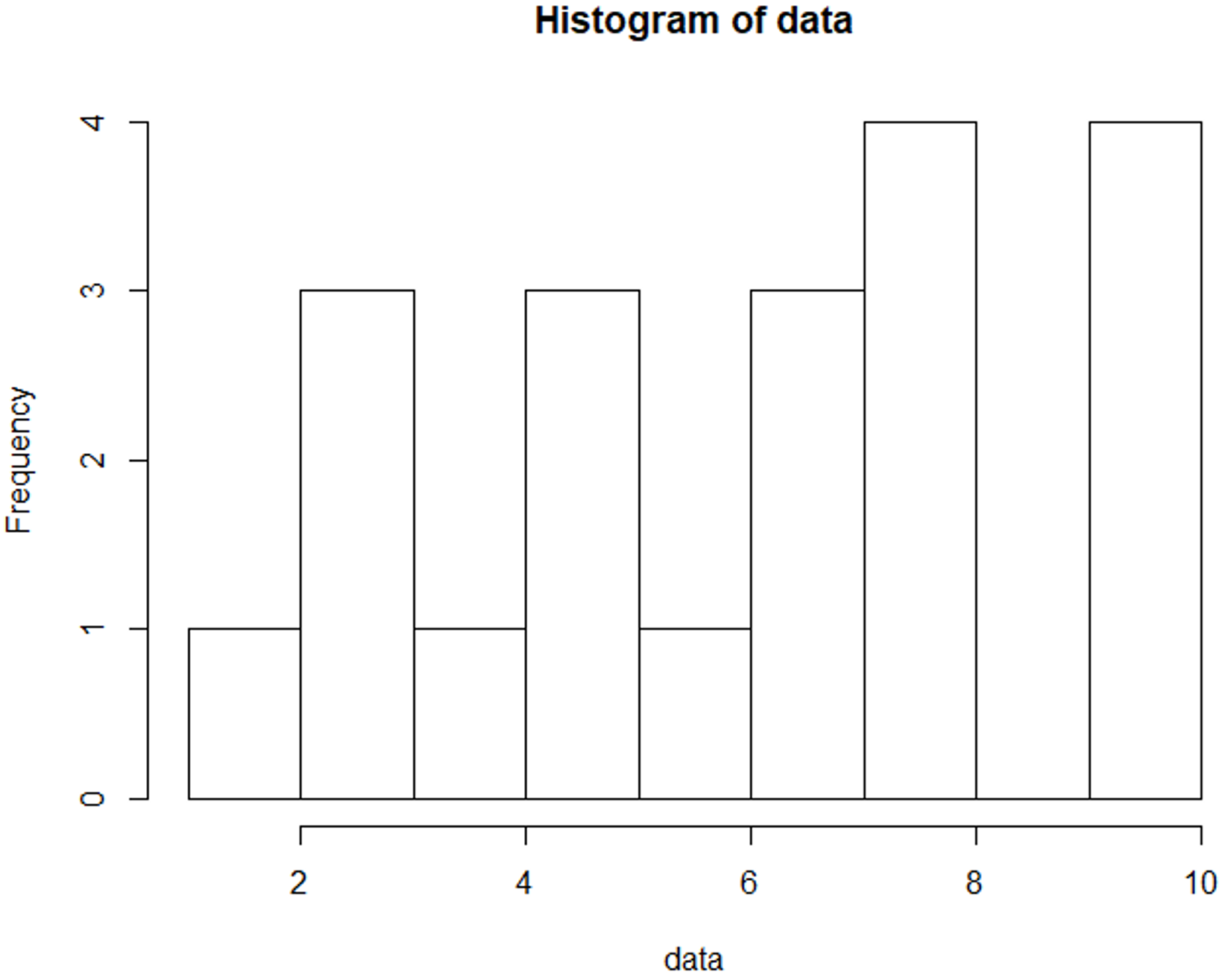
Math and Statistics For Data Science – Histogram – Edureka

So far, you’ve learned about Descriptive statistics, now let’s talk a little bit about Inferential Statistics.

Understanding Inferential Analysis

Statisticians use hypothesis testing to formally check whether the hypothesis is accepted or rejected. Hypothesis testing is an Inferential Statistical technique used to determine whether there is enough evidence in a data sample to infer that a certain condition holds true for an entire population.

To under the characteristics of a general population, we take a random sample and analyze the properties of the sample. We test whether or not the identified conclusion represents the population accurately and finally we interpret their results. Whether or not to accept the hypothesis depends upon the percentage value that we get from the hypothesis.

To better understand this, let’s look at an example.

Consider four boys, Nick, John, Bob and Harry who were caught bunking a class. They were asked to stay back at school and clean their classroom as a punishment.

Inferential Analysis – Math And Statistics For Data Science – Edureka

So, John decided that the four of them would take turns to clean their classroom. He came up with a plan of writing each of their names on chits and putting them in a bowl. Every day they had to pick up a name from the bowl and that person must clean the class.

Now it has been three days and everybody’s name has come up, except John’s! Assuming that this event is completely random and free of bias, what is the probability of John not cheating?

Let’s begin by calculating the probability of John not being picked for a day:

P(John not picked for a day) = 3/4 = 75%

The probability here is 75%, which is fairly high. Now, if John is not picked for three days in a row, the probability drops down to 42%

P(John not picked for 3 days) = 3/4 ×3/4× 3/4 = 0.42 (approx)

Now, let’s consider a situation where John is not picked for 12 days in a row! The probability drops down to 3.2%. Thus, the probability of John cheating becomes fairly high.

P(John not picked for 12 days) = (3/4) ^12 = 0.032 <?.??

In order for statisticians to come to a conclusion, they define what is known as a threshold value. Considering the above situation, if the threshold value is set to 5%, it would indicate that, if the probability lies below 5%, then John is cheating his way out of detention. But if the probability is above the threshold value, then John is just lucky, and his name isn’t getting picked.

The probability and hypothesis testing give rise to two important concepts, namely:

• Null Hypothesis: Result is no different from assumption.
• Alternate Hypothesis: Result disproves the assumption.

Therefore, in our example, if the probability of an event occurring is less than 5%, then it is a biased event, hence it approves the alternate hypothesis.

Inferential Statistics In R

In this demo, we’ll be using the gapminder data set to perform hypothesis testing. The gapminder data set contains a list of 142 countries, with their respective values for life expectancy, GDP per capita, and population, every five years, from 1952 to 2007.

We’ll begin by downloading the gapminder package and loading it into our R environment:

#Install and Load gapminder package
install.packages("gapminder")
library(gapminder)
data("gapminder")

Now, let’s take a look at our data set by using the View() function in R:

#Display gapminder dataset
View(gapminder)

Here’s a quick look at our data set:

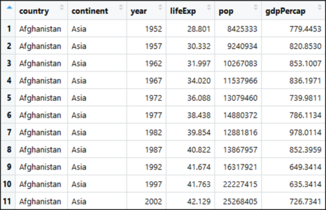
gapminder Data Set – Math And Statistics For Data Science – Edureka

The next step is to load the infamous dplyr package provided by R. We’re specifically looking to use the pipe (%>%) operator in the dplyr package. For those of you who don’t know what the pipe operator does, it basically allows you to pipe your data from the left-hand side into the data at the right-hand side of the pipe. It’s quite self-explanatory.

#Install and Load dplyr package
install.packages("dplyr")
library(dplyr)

Our next step is to compare the life expectancy of two places (Ireland and South Africa) and perform the t-test to check if the comparison follows a Null Hypothesis or an Alternate Hypothesis.

#Comparing the variance in life expectancy in South Africa & Ireland
df1 <-gapminder %>%
select(country, lifeExp) %>%
filter(country == "South Africa" | country =="Ireland")

So, after you apply the t-test to the data frame (df1), and compare the life expectancy, you can see the below results:

#Perform t-test

t.test(data = df1, lifeExp ~ country)

Welch Two Sample t-test

data: lifeExp by country
t = 10.067, df = 19.109, p-value = 4.466e-09
alternative hypothesis: true difference in means is not equal to 0
95 percent confidence interval:
15.07022 22.97794
sample estimates:
mean in group Ireland mean in group South Africa
73.01725              53.99317

Notice the mean in group Ireland and in South Africa, you can see that life expectancy almost differs by a scale of 20. Now we need to check if this difference in the value of life expectancy in South Africa and Ireland is actually valid and not just by pure chance. For this reason, the t-test is carried out.

Pay special attention to the p-value also known as the probability value. p-value is a very important measurement when it comes to ensuring the significance of a model. A model is said to be statistically significant only when the p-value is less than the pre-determined statistical significance level, which is ideally 0.05. As you can see from the output, the p value is 4.466e-09 which is an extremely small value.

In the summary of the model, notice another important parameter called the t-value. A larger t-value suggests that the alternate hypothesis is true and that the difference in life expectancy is not equal to zero by pure luck. Hence in our case, the null hypothesis is disapproved.

To conclude the demo, we’ll be plotting a graph for each continent, such that the graph shows how the life expectancy for each continent varies with the respective GDP per capita for that continent.

#Plotting a gdpPercap vs lifeExp graph for each continent
#Install and Load ggplot2 package
install.packages("ggplot2")
library(ggplot2)
gapminder%>%
filter(gdpPercap < 50000) %>%
ggplot(aes(x=log(gdpPercap), y=lifeExp, col=continent, size=pop))+
geom_point(alpha=0.3)+
geom_smooth(method = lm)+
facet_wrap(~continent)

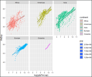
Plot – Math And Statistics For Data Science – Edureka

In the above illustration, you can almost see a linear variance in the life expectancy for each continent with respect to the GDP per capita. This also shows how well the R language can be used for Statistical Analysis.

Now that you know the Stats behind Data Science, I’m sure you’re curious to learn more about Data Science and Machine Learning. Here’s a list of blogs that you can refer after this:

1. A Comprehensive Guide To R For Data Science
2. Top 45 Data Science Interview Questions You Must Prepare In 2019
3. Data Science vs Machine Learning – What’s The Difference?
4. How To Learn Data Science?

With this, we come to the end of this blog. If you have any queries regarding this topic, please leave a comment below and we’ll get back to you.

Stay tuned for more blogs on trending technologies.

Innovative AI technology, instant language understanding with ChatGPT training course online.

If you are looking for online structured training in Data Science, Edureka! has a specially curated Data Science Course masters program that helps you gain expertise in Statistics, Data Wrangling, Exploratory Data Analysis, Machine Learning Algorithms like K-Means Clustering, Decision Trees, Random Forest, Naive Bayes. You’ll learn the concepts of Time Series, Text Mining, and an introduction to Deep Learning as well. New batches for this course are starting soon!!

Also, If you are looking for online structured training in Data Science, edureka! has a specially curated Data Science PG Program that helps you gain expertise in Statistics, Data Wrangling, Exploratory Data Analysis, and Machine Learning Algorithms like K-Means Clustering, Decision Trees, Random Forest, and Naive Bayes. You’ll learn the concepts of Time Series, Text Mining, and an introduction to Deep Learning as well. New batches for this course are starting soon!!