
Data Science with Python Certification Course
- 132k Enrolled Learners
- Weekend
- Live Class
(49300)


 Copy Link!
Linear Discriminant Analysis is a very popular Machine Learning technique that is used to solve classification problems. In this article we will try to understand the intuition and mathematics behind this technique. An example of implementation of LDA in R is also provided.
Linear Discriminant Analysis is based on the following assumptions:
The dependent variable Y is discrete. In this article we will assume that the dependent variable is binary and takes class values {+1, -1}. The probability of a sample belonging to class +1, i.e P(Y = +1) = p. Therefore, the probability of a sample belonging to class -1 is 1-p.
The independent variable(s) X come from gaussian distributions. The mean of the gaussian distribution depends on the class label Y. i.e. if Yi = +1, then the mean of Xi is 𝜇+1, else it is 𝜇-1. The variance 𝜎2 is the same for both classes. Mathematically speaking, X|(Y = +1) ~ N(𝜇+1, 𝜎2) and X|(Y = -1) ~ N(𝜇-1, 𝜎2), where N denotes the normal distribution.
With this information it is possible to construct a joint distribution P(X,Y) for the independent and dependent variable. Therefore, LDA belongs to the class of Generative Classifier Models. A closely related generative classifier is Quadratic Discriminant Analysis(QDA). It is based on all the same assumptions of LDA, except that the class variances are different.
Let us continue with Linear Discriminant Analysis article and see
Consider the class conditional gaussian distributions for X given the class Y. The below figure shows the density functions of the distributions. In this figure, if Y = +1, then the mean of X is 10 and if Y = -1, the mean is 2. The variance is 2 in both cases.

Now suppose a new value of X is given to us. Lets just denote it as xi. The task is to determine the most likely class label for this xi, i.e. yi. For simplicity assume that the probability p of the sample belonging to class +1 is the same as that of belonging to class -1, i.e. p=0.5.
Intuitively, it makes sense to say that if xi is closer to 𝜇+1 than it is to 𝜇-1, then it is more likely that yi = +1. More formally, yi = +1 if:
|xi – 𝜇+1| < |xi – 𝜇-1|
Normalizing both sides by the standard deviation:
|xi – 𝜇+1|/𝜎 < |xi – 𝜇-1|/𝜎
Squaring both sides:
(xi – 𝜇+1)2/𝜎2 < (xi – 𝜇-1)2/𝜎2
xi2/𝜎2 + 𝜇+12/𝜎2 – 2 xi𝜇+1/𝜎2 < xi2/𝜎2 + 𝜇-12/𝜎2 – 2 xi𝜇-1/𝜎2
2 xi (𝜇-1 – 𝜇+1)/𝜎2 – (𝜇-12/𝜎2 – 𝜇+12/𝜎2) < 0
-2 xi (𝜇-1 – 𝜇+1)/𝜎2 + (𝜇-12/𝜎2 – 𝜇+12/𝜎2) > 0
The above expression is of the form bxi + c > 0 where b = -2(𝜇-1 – 𝜇+1)/𝜎2 and c = (𝜇-12/𝜎2 – 𝜇+12/𝜎2).
It is apparent that the form of the equation is linear, hence the name Linear Discriminant Analysis.
Let us continue with Linear Discriminant Analysis article and see,
The mathematical derivation of the expression for LDA is based on concepts like Bayes Rule and Bayes Optimal Classifier. Interested readers are encouraged to read more about these concepts.
We will provide the expression directly for our specific case where Y takes two classes {+1, -1}. We will also extend the intuition shown in the previous section to the general case where X can be multidimensional. Let’s say that there are k independent variables. In this case, the class means 𝜇-1 and 𝜇+1 would be vectors of dimensions k*1 and the variance-covariance matrix 𝜮 would be a matrix of dimensions k*k.
The classifier function is given as
Y = h(X) = sign(bTX + c)
Where,
b = -2 𝜮 -1(𝜇-1 – 𝜇+1)
c = 𝜇-1T𝜮 -1𝜇-1 – 𝜇-1T𝜮 -1𝜇-1 -2 ln{(1-p)/p}
The sign function returns +1 if the expression bTx + c > 0, otherwise it returns -1. The natural log term in c is present to adjust for the fact that the class probabilities need not be equal for both the classes, i.e. p could be any value between (0, 1), and not just 0.5.
Given a dataset with N data-points (x1, y1), (x2, y2), … (xn, yn), we need to estimate p, 𝜇-1, 𝜇+1 and 𝜮. A statistical estimation technique called Maximum Likelihood Estimation is used to estimate these parameters. The expressions for the above parameters are given below.
𝜇+1= (1/N+1) * 𝚺i:yi=+1 xi
𝜇-1 = (1/N-1) * 𝚺i:yi=-1 xi
p = N+1/N
𝜮 = (1/N) * 𝚺i=1:N(xi – 𝜇i)(xi – 𝜇i)T
Where N+1 = number of samples where yi = +1 and N-1 = number of samples where yi = -1.
With the above expressions, the LDA model is complete. One can estimate the model parameters using the above expressions and use them in the classifier function to get the class label of any new input value of independent variable X.
Let us continue with Linear Discriminant Analysis article and see
The following code generates a dummy data set with two independent variables X1 and X2 and a dependent variable Y. For X1 and X2, we will generate sample from two multivariate gaussian distributions with means 𝜇-1= (2, 2) and 𝜇+1= (6, 6). 40% of the samples belong to class +1 and 60% belong to class -1, therefore p = 0.4.
library(ggplot2)
library(MASS)
library(mvtnorm)
#Variance Covariance matrix for random bivariate gaussian sample
var_covar = matrix(data = c(1.5, 0.3, 0.3, 1.5), nrow=2)
#Random bivariate gaussian samples for class +1
Xplus1 <- rmvnorm(400, mean = c(6, 6), sigma = var_covar)
# Random bivariate gaussian samples for class -1
Xminus1 <- rmvnorm(600, mean = c(2, 2), sigma = var_covar)
#Samples for the dependent variable
Y_samples <- c(rep(1, 400), rep(-1, 600))
#Combining the independent and dependent variables into a dataframe
dataset <- as.data.frame(cbind(rbind(Xplus1, Xminus1), Y_samples))
colnames(dataset) <- c("X1", "X2", "Y")
dataset$Y <- as.character(dataset$Y)
#Plot the above samples and color by class labels
ggplot(data = dataset)+
geom_point(aes(X1, X2, color = Y))
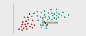
 In the above figure, the blue dots represent samples from class +1 and the red ones represent the sample from class -1. There is some overlap between the samples, i.e. the classes cannot be separated completely with a simple line. In other words they are not perfectly linearly separable.
We will now train a LDA model using the above data.
#Train the LDA model using the above dataset
lda_model <- lda(Y ~ X1 + X2, data = dataset)
#Print the LDA model
lda_model
Output:
Prior probabilities of groups:
-1 1
0.6 0.4
Group means:
X1 X2
-1 1.928108 2.010226
1 5.961004 6.015438
Coefficients of linear discriminants:
LD1
X1 0.5646116
X2 0.5004175
As one can see, the class means learnt by the model are (1.928108, 2.010226) for class -1 and (5.961004, 6.015438) for class +1. These means are very close to the class means we had used to generate these random samples. The prior probability for group +1 is the estimate for the parameter p. The b vector is the linear discriminant coefficients.
We will now use the above model to predict the class labels for the same data.
#Predicting the class for each sample in the above dataset using the LDA model
y_pred <- predict(lda_model, newdata = dataset)$class
#Adding the predictions as another column in the dataframe
dataset$Y_lda_prediction <- as.character(y_pred)
#Plot the above samples and color by actual and predicted class labels
dataset$Y_actual_pred <- paste(dataset$Y, dataset$Y_lda_prediction, sep=",")
ggplot(data = dataset)+
geom_point(aes(X1, X2, color = Y_actual_pred))</p>
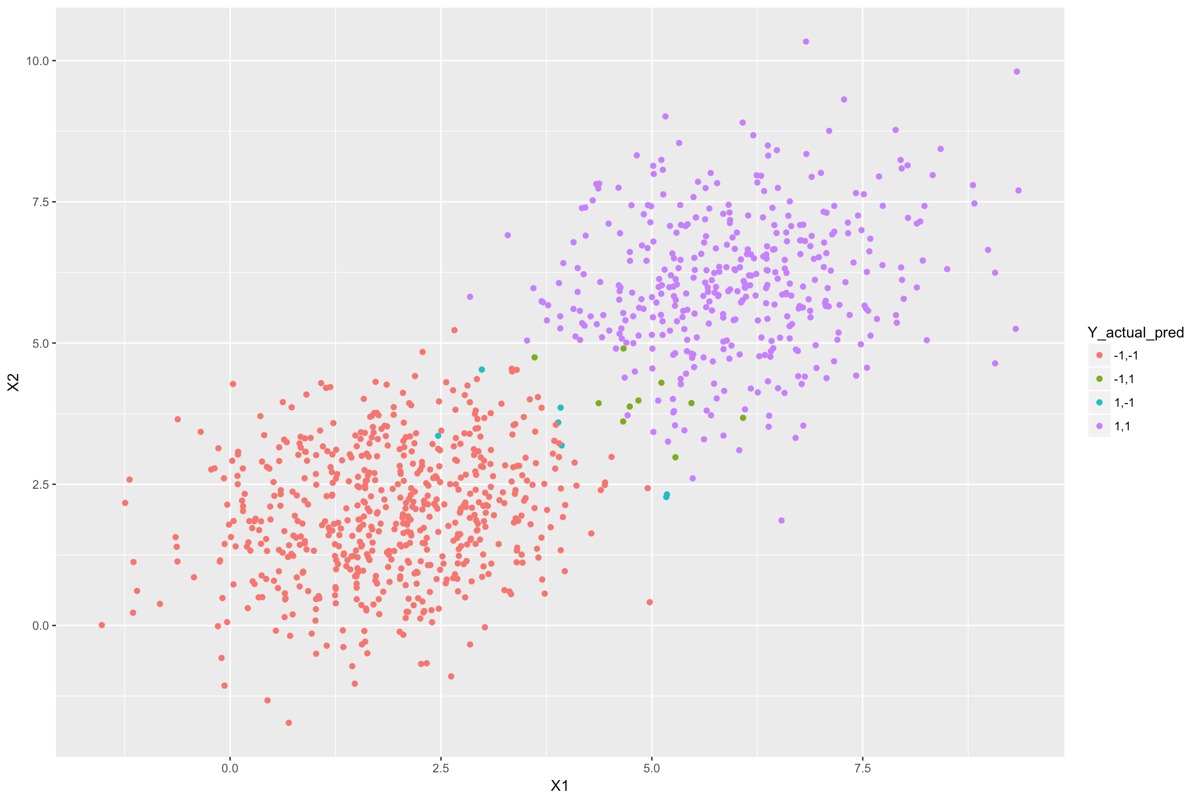 In the above figure, the purple samples are from class +1 that were classified correctly by the LDA model. Similarly, the red samples are from class -1 that were classified correctly. The blue ones are from class +1 but were classified incorrectly as -1. The green ones are from class -1 which were misclassified as +1. The misclassifications are happening because these samples are closer to the other class mean (centre) than their actual class mean.
This brings us to the end of this article, check out the R training by Edureka, a trusted online learning company with a network of more than 250,000 satisfied learners spread across the globe. Edureka’s Data Analytics with R training will help you gain expertise in R Programming, Data Manipulation, Exploratory Data Analysis, Data Visualization, Data Mining, Regression, Sentiment Analysis and using R Studio for real life case studies on Retail, Social Media.
Got a question for us? Please mention it in the comments section of this article and we will get back to you as soon as possible.


 Thank you for registering Join Edureka Meetup community for 100+ Free Webinars each month JOIN MEETUP GROUP