A 101 Guide On The Least Squares Regression Method

With Machine Learning and Artificial Intelligence booming the IT market it has become essential to learn the fundamentals of these trending technologies. This blog on Least Squares Regression Method will help you understand the math behind Regression Analysis and how it can be implemented using Python.

To get in-depth knowledge of Artificial Intelligence and Machine Learning, you can enroll for live Machine Learning Engineer Master Program by Edureka with 24/7 support and lifetime access.

Here’s a list of topics that will be covered in this blog:

1. What Is the Least Squares Method?
2. Line Of Best Fit
3. Steps to Compute the Line Of Best Fit
4. The least-squares regression method with an example
5. A short python script to implement Linear Regression

What is the Least Squares Regression Method?

The least-squares regression method is a technique commonly used in Regression Analysis. It is a mathematical method used to find the best fit line that represents the relationship between an independent and dependent variable. 

To understand the least-squares regression method lets get familiar with the concepts involved in formulating the line of best fit.

🐍 Ready to Unleash the Power of Python? Sign Up for Edureka’s Comprehensive Online Python online course with certificate with access to hundreds of Python learning Modules and 24/7 technical support.

What is the Line Of Best Fit?

Line of best fit is drawn to represent the relationship between 2 or more variables. To be more specific, the best fit line is drawn across a scatter plot of data points in order to represent a relationship between those data points.

Regression analysis makes use of mathematical methods such as least squares to obtain a definite relationship between the predictor variable (s) and the target variable. The least-squares method is one of the most effective ways used to draw the line of best fit. It is based on the idea that the square of the errors obtained must be minimized to the most possible extent and hence the name least squares method.

If we were to plot the best fit line that shows the depicts the sales of a company over a period of time, it would look something like this:

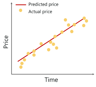
Notice that the line is as close as possible to all the scattered data points. This is what an ideal best fit line looks like.

To better understand the whole process let’s see how to calculate the line using the Least Squares Regression.

Steps to calculate the Line of Best Fit

To start constructing the line that best depicts the relationship between variables in the data, we first need to get our basics right. Take a look at the equation below:

Surely, you’ve come across this equation before. It is a simple equation that represents a straight line along 2 Dimensional data, i.e. x-axis and y-axis. To better understand this, let’s break down the equation:

• y: dependent variable
• m: the slope of the line
• x: independent variable
• c: y-intercept

So the aim is to calculate the values of slope, y-intercept and substitute the corresponding ‘x’ values in the equation in order to derive the value of the dependent variable.

Let’s see how this can be done.

As an assumption, let’s consider that there are ‘n’ data points.

Step 1: Calculate the slope ‘m’ by using the following formula:

Step 2: Compute the y-intercept (the value of y at the point where the line crosses the y-axis):

Step 3: Substitute the values in the final equation:

Simple, isn’t it?

Now let’s look at an example and see how you can use the least-squares regression method to compute the line of best fit.

Least Squares Regression Example

Consider an example. Tom who is the owner of a retail shop, found the price of different T-shirts vs the number of T-shirts sold at his shop over a period of one week.

He tabulated this like shown below:

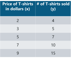
Let us use the concept of least squares regression to find the line of best fit for the above data.

Step 1: Calculate the slope ‘m’ by using the following formula:

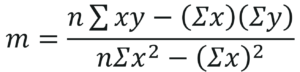
After you substitute the respective values, m = 1.518 approximately.

Step 2: Compute the y-intercept value

After you substitute the respective values, c = 0.305 approximately.

Step 3: Substitute the values in the final equation

Once you substitute the values, it should look something like this:

Let’s construct a graph that represents the y=mx + c line of best fit:

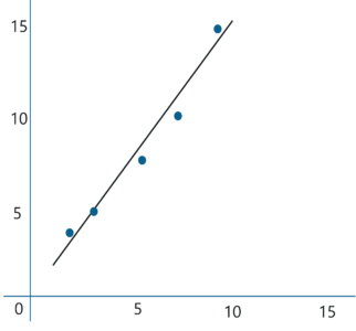
Now Tom can use the above equation to estimate how many T-shirts of price $8 can he sell at the retail shop.

y = 1.518 x 8 + 0.305 = 12.45 T-shirts

This comes down to 13 T-shirts! That’s how simple it is to make predictions using Linear Regression.

Now let’s try to understand based on what factors can we confirm that the above line is the line of best fit.

The least squares regression method works by minimizing the sum of the square of the errors as small as possible, hence the name least squares. Basically the distance between the line of best fit and the error must be minimized as much as possible. This is the basic idea behind the least squares regression method.

A few things to keep in mind before implementing the least squares regression method is:

• The data must be free of outliers because they might lead to a biased and wrongful line of best fit.
• The line of best fit can be drawn iteratively until you get a line with the minimum possible squares of errors.
• This method works well even with non-linear data.
• Technically, the difference between the actual value of ‘y’ and the predicted value of ‘y’ is called the Residual (denotes the error).

Now let’s wrap up by looking at a practical implementation of linear regression using Python.

Least Squares Regression In Python

In this section, we will be running a simple demo to understand the working of Regression Analysis using the least squares regression method. A short disclaimer, I’ll be using Python for this demo, if you’re not familiar with the language, you can go through the following blogs:

1. Python Tutorial – A Complete Guide to Learn Python Programming
2. Python Programming Language – Headstart With Python Basics
3. A Beginners Guide To Python Functions
4. Python for Data Science

Problem Statement: To apply Linear Regression and build a model that studies the relationship between the head size and the brain weight of an individual.

Data Set Description: The data set contains the following variables:

• Gender: Male or female represented as binary variables
• Age: Age of an individual
• Head size in cm^3: An individuals head size in cm^3
• Brain weight in grams: The weight of an individual’s brain measured in grams

These variables need to be analyzed in order to build a model that studies the relationship between the head size and brain weight of an individual.

Logic: To implement Linear Regression in order to build a model that studies the relationship between an independent and dependent variable. The model will be evaluated by using least square regression method where RMSE and R-squared will be the model evaluation parameters.

Let’s get started!

Step 1: Import the required libraries 

import numpy as np
import pandas as pd
import matplotlib.pyplot as plt

Step 2: Import the data set

# Reading Data
data = pd.read_csv('C:UsersNeelTempDesktopheadbrain.csv')
print(data.shape)
(237, 4)
print(data.head())
   Gender  Age Range  Head Size(cm^3)  Brain Weight(grams)
0       1          1             4512                 1530
1       1          1             3738                 1297
2       1          1             4261                 1335
3       1          1             3777                 1282
4       1          1             4177                 1590

Step 3: Assigning ‘X’ as independent variable and ‘Y’ as dependent variable

# Coomputing X and Y
X = data['Head Size(cm^3)'].values
Y = data['Brain Weight(grams)'].values

Next, in order to calculate the slope and y-intercept we first need to compute the means of ‘x’ and ‘y’. This can be done as shown below:

# Mean X and Y
mean_x = np.mean(X)
mean_y = np.mean(Y)

# Total number of values
n = len(X)

Step 4: Calculate the values of the slope and y-intercept

# Using the formula to calculate 'm' and 'c'
numer = 0
denom = 0
for i in range(n):
numer += (X[i] - mean_x) * (Y[i] - mean_y)
denom += (X[i] - mean_x) ** 2
m = numer / denom
c = mean_y - (m * mean_x)

# Printing coefficients
print("Coefficients")
print(m, c)

Coefficients
0.26342933948939945 325.57342104944223

The above coefficients are our slope and intercept values respectively. On substituting the values in the final equation, we get:

Brain Weight = 325.573421049 + 0.263429339489 * Head Size

As simple as that, the above equation represents our linear model.

Now let’s plot this graphically.

Step 5: Plotting the line of best fit

# Plotting Values and Regression Line

max_x = np.max(X) + 100
min_x = np.min(X) - 100

# Calculating line values x and y
x = np.linspace(min_x, max_x, 1000)
y = c + m * x

# Ploting Line
plt.plot(x, y, color='#58b970', label='Regression Line')
# Ploting Scatter Points
plt.scatter(X, Y, c='#ef5423', label='Scatter Plot')

plt.xlabel('Head Size in cm3')
plt.ylabel('Brain Weight in grams')
plt.legend()
plt.show()

Step 6: Model Evaluation

The model built is quite good given the fact that our data set is of a small size. It’s time to evaluate the model and see how good it is for the final stage i.e., prediction. To do that we will use the Root Mean Squared Error method that basically calculates the least-squares error and takes a root of the summed values.

Mathematically speaking, Root Mean Squared Error is nothing but the square root of the sum of all errors divided by the total number of values. This is the formula to calculate RMSE:

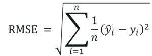
In the above equation, yi​^​ is the i^th predicted output value. Let’s see how this can be done using Python.

# Calculating Root Mean Squares Error
rmse = 0
for i in range(n):
    y_pred = c + m * X[i]
    rmse += (Y[i] - y_pred) ** 2
rmse = np.sqrt(rmse/n)
print("RMSE")
print(rmse)
RMSE
72.1206213783709

Another model evaluation parameter is the statistical method called, R-squared value that measures how close the data are to the fitted line of best
fit.

Mathematically, it can be calculated as:

$Where,$

• SSt​ is the total sum of squares
• SSr​ is the total sum of squares of residuals

The value of R-squared ranges between 0 and 1. A negative value denoted that the model is weak and the prediction thus made are wrong and biased. In such situations, it’s essential that you analyze all the predictor variables and look for a variable that has a high correlation with the output. This step usually falls under EDA or Exploratory Data Analysis.

Let’s not get carried away. Here’s how you implement the computation of R-squared in Python:

# Calculating R2 Score
ss_tot = 0
ss_res = 0
for i in range(n):
    y_pred = c + m * X[i]
    ss_tot += (Y[i] - mean_y) ** 2
    ss_res += (Y[i] - y_pred) ** 2
r2 = 1 - (ss_res/ss_tot)
print("R2 Score")
print(r2)
R2 Score
0.6393117199570003

As you can see our R-squared value is quite close to 1, this denotes that our model is doing good and can be used for further predictions.

So that was the entire implementation of Least Squares Regression method using Python. Now that you know the math behind Regression Analysis, I’m sure you’re curious to learn more. Here are a few blogs to get you started:

1. A Complete Guide To Maths And Statistics For Data Science
2. All You Need To Know About Statistics And Probability
3. Introduction To Markov Chains With Examples – Markov Chains With Python
4. How To Implement Bayesian Networks In Python? – Bayesian Networks Explained With Examples

With this, we come to the end of this blog. If you have any queries regarding this topic, please leave a comment below and we’ll get back to you.

If you wish to enroll for a complete course on Artificial Intelligence and Machine Learning, Edureka has a specially curated Machine Learning Engineer Master Program that will make you proficient in techniques like Supervised Learning, Unsupervised Learning, and Natural Language Processing. It includes training on the latest advancements and technical approaches in Artificial Intelligence & Machine Learning such as Deep Learning, Graphical Models and Reinforcement Learning.