
Data Science with Python Certification Course
- 132k Enrolled Learners
- Weekend
- Live Class
(49300)


 Copy Link!
_1648290501.jpg)
With the amount of data that we’re generating, the need for advanced Machine Learning Algorithms has increased. One such algorithm is the K Nearest Neighbour algorithm. In this blog on KNN Algorithm In R, you will understand how the KNN algorithm works and its implementation using the R Language.
To get in-depth knowledge on Data Science, you can enroll for live Data Science Certification Training by Edureka with 24/7 support and lifetime access.
The following topics will be covered in this KNN Algorithm In R blog:
It is essential that you know Machine Learning basics before you get started with this KNN Algorithm In R blog. Here’s a list of Machine learning blogs to get you started:
To get an in-depth understanding of the KNN Algorithm In R, you can go through this video recorded by our Machine Learning experts.
This Edureka video on “KNN algorithm using R”, will help you learn about the KNN algorithm in depth, you’ll also see how KNN is used to solve real-world problems.
Let’s try to understand the KNN algorithm with a simple example. Let’s say we want a machine to distinguish between images of cats & dogs. To do this we must input a dataset of cat and dog images and we have to train our model to detect the animals based on certain features. For example, features such as pointy ears can be used to identify cats and similarly we can identify dogs based on their long ears.
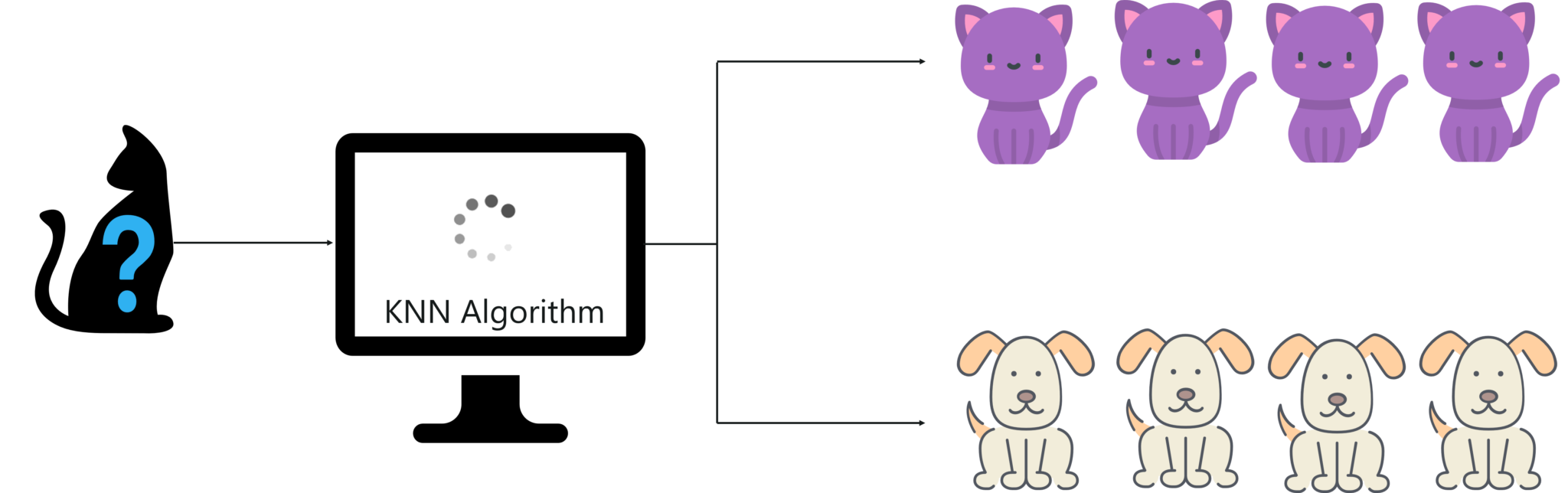
What is KNN Algorithm? – KNN Algorithm In R – Edureka
After studying the dataset during the training phase, when a new image is given to the model, the KNN algorithm will classify it into either cats or dogs depending on the similarity in their features. So if the new image has pointy ears, it will classify that image as a cat because it is similar to the cat images. In this manner, the KNN algorithm classifies data points based on how similar they are to their neighboring data points.
Now let’s discuss the features of the KNN algorithm.
The KNN algorithm has the following features:
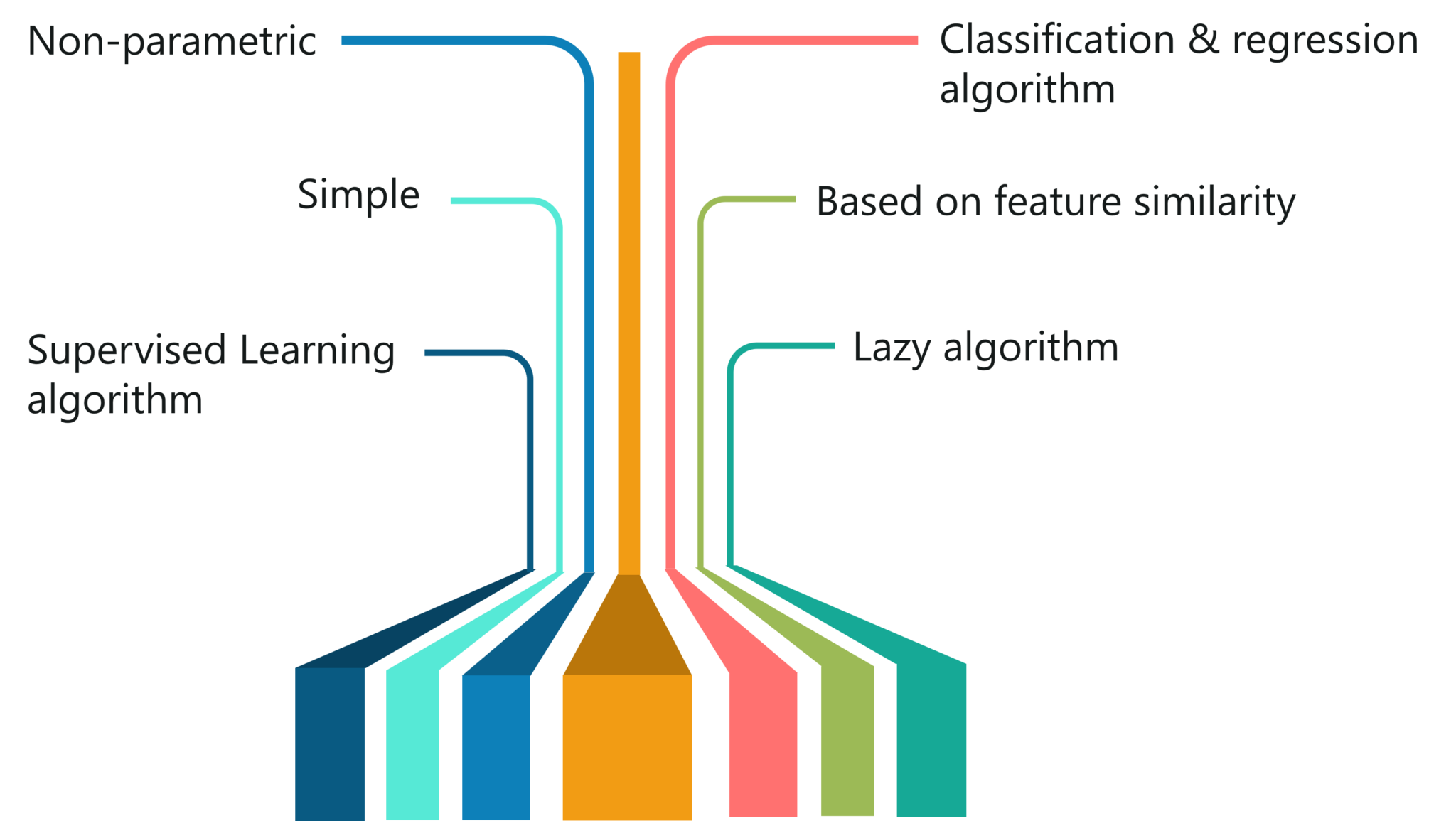
Features of KNN – KNN Algorithm In R – Edureka
To make you understand how KNN algorithm works, let’s consider the following scenario:
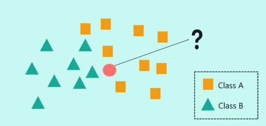
How does KNN Algorithm work? – KNN Algorithm In R – Edureka
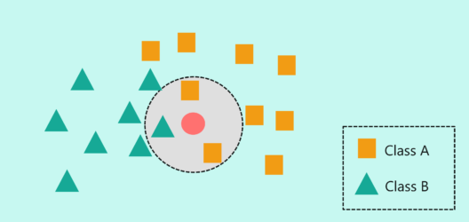
How does KNN Algorithm work? – KNN Algorithm In R – Edureka

How does KNN Algorithm work? – KNN Algorithm In R – Edureka
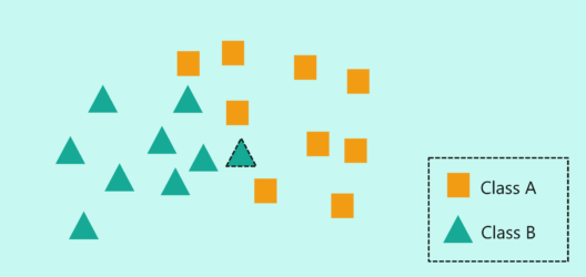
How does KNN Algorithm work? – KNN Algorithm In R – Edureka
In practice, there’s a lot more to consider while implementing the KNN algorithm. This will be discussed in the demo section of the blog.
Earlier I mentioned that KNN uses Euclidean distance as a measure to check the distance between a new data point and its neighbors, let’s see how.
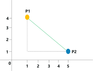
Euclidian Distance – KNN Algorithm In R – Edureka

Euclidian Distance Calculations – KNN Algorithm In R – Edureka
It is as simple as that! KNN makes use of simple measure in order to solve complex problems, this is one of the reasons why KNN is such a commonly used algorithm.
To sum it up, let’s look at the pseudocode for KNN Algorithm.
Consider the set, (Xi, Ci),
The condition, Ci ∈ {1, 2, 3, ……, c} is acceptable for all values of ‘i’ by assuming that the total number of classes is denoted by ‘c’.
Now let’s pretend that there’s a data point ‘x’ whose output class needs to be predicted. This can be done by using the K-Nearest Neighbour (KNN) Algorithm.
Calculate D(x, xi), where 'i' =1, 2, ….., n and 'D' is the Euclidean measure between the data points.
The calculated Euclidean distances must be arranged in ascending order.
Initialize k and take the first k distances from the sorted list.
Figure out the k points for the respective k distances.
Calculate ki, which indicates the number of data points belonging to the ith class among k points i.e. k ≥ 0
If ki >kj ∀ i ≠ j; put x in class i.
The above pseudocode can be used for solving a classification problem by using the KNN Algorithm.
Before we get into the practical implementation of KNN, let’s look at a real-world use case of the KNN algorithm.
Surely you have shopped on Amazon! Have you ever noticed that when you buy a product, Amazon gives you a list of recommendations based on your purchase? Not only this, Amazon displays a section which says, ‘customers who bought this item also bought this.. ‘.
Machine learning plays a huge role in Amazon’s recommendation system. The logic behind a recommendation engine is to suggest products to customers based on other customers who have a similar shopping behavior.

KNN Use Case- KNN Algorithm In R – Edureka
Consider an example, let’s say that a customer A who loves mystery novels bought the Game Of Thrones and Lord Of The Rings book series. Now a couple of weeks later, another customer B who reads books of the same genre buys Lord Of The Rings. He does not buy the Game of Thrones book series, but Amazon recommends it customer B since his shopping behaviors and his choice in books is quite similar to customer A.
Therefore, Amazon recommends products to customers based on how similar their shopping behaviors are. This similarity can be understood by implementing the KNN algorithm which is mainly based on feature similarity.
Now that you know how KNN works and how it is used in real-world applications, let’s discuss the implementation of KNN using the R language. If you’re not familiar with the R language, you can go through this video recorded by our Machine Learning experts.
This Edureka video on R Programming Tutorial For Beginners will help you in understanding the fundamentals of R and will help you build a strong foundation in R.
Problem Statement: To study a bank credit dataset and build a Machine Learning model that predicts whether an applicant’s loan can be approved or not based on his socio-economic profile.
Dataset Description: The bank credit dataset contains information about 1000s of applicants. This includes their account balance, credit amount, age, occupation, loan records, etc. By using this data, we can predict whether or not to approve the loan of an applicant.

Dataset – KNN Algorithm In R – Edureka
Logic: This problem statement can be solved using the KNN algorithm that will classify the applicant’s loan request into two classes:
Now that you know the objective of this project, let’s get started with the coding part.
Step 1: Import the dataset
#Import the dataset
loan <- read.csv("C:/Users/zulaikha/Desktop/DATASETS/knn dataset/credit_data.csv")
After importing the dataset, let’s take a look at the structure of the dataset:
str(loan)
'data.frame': 1000 obs. of 21 variables:
$ Creditability : int 1 1 1 1 1 1 1 1 1 1 ...
$ Account.Balance : int 1 1 2 1 1 1 1 1 4 2 ...
$ Duration.of.Credit..month. : int 18 9 12 12 12 10 8 6 18 24 ...
$ Payment.Status.of.Previous.Credit: int 4 4 2 4 4 4 4 4 4 2 ...
$ Purpose : int 2 0 9 0 0 0 0 0 3 3 ...
$ Credit.Amount : int 1049 2799 841 2122 2171 2241 3398 1361 1098 3758 ...
$ Value.Savings.Stocks : int 1 1 2 1 1 1 1 1 1 3 ...
$ Length.of.current.employment : int 2 3 4 3 3 2 4 2 1 1 ...
$ Instalment.per.cent : int 4 2 2 3 4 1 1 2 4 1 ...
$ Sex...Marital.Status : int 2 3 2 3 3 3 3 3 2 2 ...
$ Guarantors : int 1 1 1 1 1 1 1 1 1 1 ...
$ Duration.in.Current.address : int 4 2 4 2 4 3 4 4 4 4 ...
$ Most.valuable.available.asset : int 2 1 1 1 2 1 1 1 3 4 ...
$ Age..years. : int 21 36 23 39 38 48 39 40 65 23 ...
$ Concurrent.Credits : int 3 3 3 3 1 3 3 3 3 3 ...
$ Type.of.apartment : int 1 1 1 1 2 1 2 2 2 1 ...
$ No.of.Credits.at.this.Bank : int 1 2 1 2 2 2 2 1 2 1 ...
$ Occupation : int 3 3 2 2 2 2 2 2 1 1 ...
$ No.of.dependents : int 1 2 1 2 1 2 1 2 1 1 ...
$ Telephone : int 1 1 1 1 1 1 1 1 1 1 ...
$ Foreign.Worker : int 1 1 1 2 2 2 2 2 1 1 ...
Note that, the ‘Creditability’ variable is our output variable or the target variable. The value of the credibility variable represents whether an applicant’s loan is approved or rejected.
Step 2: Data Cleaning
From the structure of the dataset, we can see that there are 21 predictor variables that will help us decide whether or not an applicant’s loan must be approved.
Some of these variables are not essential in predicting the loan of an applicant, for example, variables such as Telephone, Concurrent. Credits, Duration.in.Current.address, Type.of.apartment, etc. Such variables must be removed because they will only increase the complexity of the Machine Learning model.
loan.subset <- loan[c('Creditability','Age..years.','Sex...Marital.Status','Occupation','Account.Balance','Credit.Amount','Length.of.current.employment','Purpose')]
In the above code snippet, I’ve filtered down the predictor variables. Now let’s take a look at how our dataset looks:
str(loan.subset)
'data.frame': 1000 obs. of 8 variables:
$ Creditability : int 1 1 1 1 1 1 1 1 1 1 ...
$ Age..years. : int 21 36 23 39 38 48 39 40 65 23 ...
$ Sex...Marital.Status : int 2 3 2 3 3 3 3 3 2 2 ...
$ Occupation : int 3 3 2 2 2 2 2 2 1 1 ...
$ Account.Balance : int 1 1 2 1 1 1 1 1 4 2 ...
$ Credit.Amount : int 1049 2799 841 2122 2171 2241 3398 1361 1098 3758 ...
$ Length.of.current.employment: int 2 3 4 3 3 2 4 2 1 1 ...
$ Purpose : int 2 0 9 0 0 0 0 0 3 3 ...
Now we have narrowed down 21 variables to 8 predictor variables that are significant for building the model.
Step 3: Data Normalization
You must always normalize the data set so that the output remains unbiased. To explain this, let’s take a look at the first few observations in our data set.
head(loan.subset)
  Creditability Age..years. Sex...Marital.Status Occupation Account.Balance Credit.Amount
1             1          21                    2          3               1          1049
2             1          36                    3          3               1          2799
3             1          23                    2          2               2           841
4             1          39                    3          2               1          2122
5             1          38                    3          2               1          2171
6             1          48                    3          2               1          2241
  Length.of.current.employment Purpose
1                            2       2
2                            3       0
3                            4       9
4                            3       0
5                            3       0
6                            2       0
Notice the Credit amount variable, its value scale is in 1000s, whereas the rest of the variables are in single digits or 2 digits. If the data isn’t normalized it will lead to a baised outcome.
#Normalization
normalize <- function(x) {
return ((x - min(x)) / (max(x) - min(x))) }
In the below code snippet, we’re storing the normalized data set in the ‘loan.subset.n’ variable and also we’re removing the ‘Credibility’ variable since it’s the response variable that needs to be predicted.
loan.subset.n <- as.data.frame(lapply(loan.subset[,2:8], normalize))
This is the normalized data set:
head(loan.subset.n)
   Age..years. Sex..Marital Occupation Account.Balance Credit.Amount
1  0.03571429   0.3333333   0.6666667    0.0000000      0.04396390
2  0.30357143   0.6666667   0.6666667    0.0000000      0.14025531
3  0.07142857   0.3333333   0.3333333    0.3333333      0.03251898
4  0.35714286   0.6666667   0.3333333    0.0000000      0.10300429
5  0.33928571   0.6666667   0.3333333    0.0000000      0.10570045
6  0.51785714   0.6666667   0.3333333    0.0000000      0.10955211
Length.of.current.employment Purpose
            0.25                0.2
            0.50                0.0
            0.75                0.9
            0.50                0.0
            0.50                0.0
            0.25                0.0
Step 4: Data Splicing
After cleaning the data set and formatting it, the next step is data splicing. Data splicing basically involves splitting the data set into training and testing data set. This is done in the following code snippet:
set.seed(123)
dat.d <- sample(1:nrow(loan.subset.n),size=nrow(loan.subset.n)*0.7,replace = FALSE) #random selection of 70% data.

train.loan <- loan.subset[dat.d,] # 70% training data
test.loan <- loan.subset[-dat.d,] # remaining 30% test data
After deriving the training and testing data set, the below code snippet is going to create a separate data frame for the ‘Creditability’ variable so that our final outcome can be compared with the actual value.
#Creating seperate dataframe for 'Creditability' feature which is our target.
train.loan_labels <- loan.subset[dat.d,1]
test.loan_labels <-loan.subset[-dat.d,1]
Step 5: Building a Machine Learning model
At this stage, we have to build a model by using the training data set. Since we’re using the KNN algorithm to build the model, we must first install the ‘class’ package provided by R. This package has the KNN function in it:
#Install class package
install.packages('class')
# Load class package
library(class)
Next, we’re going to calculate the number of observations in the training data set. The reason we’re doing this is that we want to initialize the value of ‘K’ in the KNN model. One of the ways to find the optimal K value is to calculate the square root of the total number of observations in the data set. This square root will give you the ‘K’ value.
#Find the number of observation
NROW(train.loan_labels)
[1] 700
So, we have 700 observations in our training data set. The square root of 700 is around 26.45, therefore we’ll create two models. One with ‘K’ value as 26 and the other model with a ‘K’ value as 27.
knn.26 <- knn(train=train.loan, test=test.loan, cl=train.loan_labels, k=26)
knn.27 <- knn(train=train.loan, test=test.loan, cl=train.loan_labels, k=27)
Step 6: Model Evaluation
After building the model, it is time to calculate the accuracy of the created models:
#Calculate the proportion of correct classification for k = 26, 27
ACC.26 <- 100 * sum(test.loan_labels == knn.26)/NROW(test.loan_labels)
ACC.27 <- 100 * sum(test.loan_labels == knn.27)/NROW(test.loan_labels)

ACC.26
[1] 67.66667

ACC.27
[1] 67.33333
As shown above, the accuracy for K = 26 is 67.66 and for K = 27 it is 67.33. We can also check the predicted outcome against the actual value in tabular form:
# Check prediction against actual value in tabular form for k=26
table(knn.26 ,test.loan_labels)

       test.loan_labels
knn.26   0     1
0        11    7
1        90   192

knn.26
[1] 1 1 1 1 1 1 1 1 1 1 1 1 1 1 1 1 1 1 1 1 1 1 1 1 1 1 1 1 1 1 1 1 1 1 1 1 1 1 1 1 1 1 1 1 1 1 1 0 1 1
[51] 1 1 1 1 1 1 1 1 1 1 1 0 0 1 1 1 1 1 1 1 1 1 1 1 1 1 1 1 1 1 1 1 1 1 1 1 1 1 1 1 1 1 1 1 1 1 1 1 1 1
[101] 1 1 1 1 1 0 1 1 1 1 1 1 1 1 1 1 1 1 1 1 1 1 1 1 1 1 1 1 1 1 1 1 1 1 1 1 1 1 1 1 1 1 1 1 1 1 1 1 1 1
[151] 1 0 1 1 1 1 1 1 1 1 1 1 1 1 1 1 1 1 1 1 1 1 1 1 1 1 1 1 1 1 1 1 0 1 1 1 0 1 1 1 1 1 1 1 1 1 1 1 1 1
[201] 1 1 1 1 1 1 1 1 1 1 1 1 0 1 1 1 1 1 1 1 0 1 1 1 1 1 1 1 1 1 1 1 1 1 1 1 1 1 0 1 1 1 1 1 1 1 1 1 1 1
[251] 0 1 1 0 1 1 1 1 1 1 1 1 1 0 1 0 1 1 1 1 1 1 1 1 0 1 1 1 1 1 0 1 1 1 1 0 1 1 1 1 1 1 0 1 1 1 1 1 1 1
Levels: 0 1
# Check prediction against actual value in tabular form for k=27
table(knn.27 ,test.loan_labels)

       test.loan_labels
knn.27    0     1
0         11    8
1         90   191

knn.27
[1] 1 1 1 1 1 1 1 1 1 1 1 1 1 1 1 1 1 1 1 1 1 1 1 1 1 1 1 1 1 1 1 1 1 1 1 1 1 1 1 1 1 1 1 1 1 1 1 0 1 1
[51] 1 1 1 1 1 1 1 1 1 1 1 0 1 1 0 1 1 1 1 1 1 1 1 1 1 1 1 1 1 1 1 1 1 1 1 1 1 1 1 1 1 1 1 1 1 1 1 1 1 1
[101] 1 1 1 1 1 0 1 1 1 1 1 1 1 1 1 1 1 1 1 1 1 1 1 1 1 1 1 1 1 1 1 1 1 1 1 1 1 1 1 1 1 1 1 1 1 1 1 1 1 1
[151] 1 0 1 1 1 1 1 1 1 1 1 1 1 1 1 1 1 1 1 1 1 1 1 1 1 1 1 1 1 1 1 1 0 1 1 1 0 1 1 1 1 1 1 1 1 1 1 1 1 1
[201] 1 1 1 1 1 0 1 1 1 1 1 1 0 1 1 1 1 1 1 1 0 1 1 1 1 1 1 1 1 1 1 1 1 1 1 1 1 1 0 1 1 1 1 1 1 1 1 1 1 1
[251] 0 1 1 0 1 1 1 1 1 1 1 1 1 0 1 0 1 1 1 1 1 1 1 1 0 1 1 1 1 1 0 1 1 1 1 0 1 1 1 1 1 1 0 1 1 1 1 1 1 1
Levels: 0 1
You can also use the confusion matrix to calculate the accuracy. To do this we must first install the infamous Caret package:
install.packages('caret')
library(caret)
Now, let’s use the confusion matrix to calculate the accuracy of the KNN model with K value set to 26:
confusionMatrix(table(knn.26 ,test.loan_labels))
Confusion Matrix and Statistics
       test.loan_labels
knn.26   0   1
     0  11   7
     1  90 192

               Accuracy : 0.6767
                 95% CI : (0.6205, 0.7293)
    No Information Rate : 0.6633
    P-Value [Acc > NIR] : 0.3365

                  Kappa : 0.0924
 Mcnemar's Test P-Value : <2e-16

            Sensitivity : 0.10891
            Specificity : 0.96482
         Pos Pred Value : 0.61111
         Neg Pred Value : 0.68085
             Prevalence : 0.33667
         Detection Rate : 0.03667
   Detection Prevalence : 0.06000
      Balanced Accuracy : 0.53687

       'Positive' Class : 0
So, from the output, we can see that our model predicts the outcome with an accuracy of 67.67% which is good since we worked with a small data set. A point to remember is that the more data (optimal data) you feed the machine, the more efficient the model will be.
Step 7: Optimization
In order to improve the accuracy of the model, you can use n number of techniques such as the Elbow method and maximum percentage accuracy graph. In the below code snippet, I’ve created a loop that calculates the accuracy of the KNN model for ‘K’ values ranging from 1 to 28. This way you can check which ‘K’ value will result in the most accurate model:
i=1
k.optm=1
for (i in 1:28){
+ knn.mod <- knn(train=train.loan, test=test.loan, cl=train.loan_labels, k=i)
+ k.optm[i] <- 100 * sum(test.loan_labels == knn.mod)/NROW(test.loan_labels)
+ k=i
+ cat(k,'=',k.optm[i],'
')
+ }
1 = 60.33333
2 = 58.33333
3 = 60.33333
4 = 61
5 = 62.33333
6 = 62
7 = 63.33333
8 = 63.33333
9 = 63.33333
10 = 64.66667
11 = 64.66667
12 = 65.33333
13 = 66
14 = 64
15 = 66.66667
16 = 67.66667
17 = 67.66667
18 = 67.33333
19 = 67.66667
20 = 67.66667
21 = 66.33333
22 = 67
23 = 67.66667
24 = 67
25 = 68
26 = 67.66667
27 = 67.33333
28 = 66.66667
From the output you can see that for K = 25, we achieve the maximum accuracy, i.e. 68%. We can also represent this graphically, like so:
#Accuracy plot
plot(k.optm, type="b", xlab="K- Value",ylab="Accuracy level")

Accuracy Plot – KNN Algorithm In R – Edureka
The above graph shows that for ‘K’ value of 25 we get the maximum accuracy. Now that you know how to build a KNN model, I’ll leave it up to you to build a model with ‘K’ value as 25.
Now that you know how the KNN algorithm works, I’m sure you’re curious to learn more about the various Machine learning algorithms. Here’s a list of blogs that covers the different types of Machine Learning algorithms in depth:
With this, we come to the end of this KNN Algorithm In R blog. I hope you found this blog informative, if you have any doubts, leave a comment and we’ll get back to you.
Stay tuned for more blogs on trending technologies.
If you are looking for online structured training in Data Science, edureka! has a specially curated Data Science course which helps you gain expertise in Statistics, Data Wrangling, Exploratory Data Analysis, Machine Learning Algorithms like K-Means Clustering, Decision Trees, Random Forest, Naive Bayes. You’ll learn the concepts of Time Series, Text Mining and an introduction to Deep Learning as well. New batches for this course are starting soon!!


 Thank you for registering Join Edureka Meetup community for 100+ Free Webinars each month JOIN MEETUP GROUP