Introduction To Machine Learning: All You Need To Know About Machine Learning

Introduction To Machine Learning:

Undoubtedly, Machine Learning is the most in-demand technology in today’s market. Its applications range from self-driving cars to predicting deadly diseases such as ALS. The high demand for Machine Learning skills is the motivation behind this blog. In this blog on Introduction To Machine Learning, you will understand all the basic concepts of Machine Learning and a Practical Implementation of Machine Learning by using the R language.

The following topics are covered in this Introduction To Machine Learning blog:

1. Need For Machine Learning
2. What Is Machine Learning?
3. Machine Learning Definitions
4. Machine Learning Process
5. Types Of Machine Learning
6. Type Of Problems Solved Using Machine Learning
7. Practical Implementation Of Machine Learning

Need For Machine Learning

Ever since the technical revolution, we’ve been generating an immeasurable amount of data. As per research, we generate around 2.5 quintillion bytes of data every single day! It is estimated that by 2020, 1.7MB of data will be created every second for every person on earth.

With the availability of so much data, it is finally possible to build predictive models that can study and analyze complex data to find useful insights and deliver more accurate results.

Top Tier companies such as Netflix and Amazon build such Machine Learning models by using tons of data in order to identify profitable opportunities and avoid unwanted risks.

Here’s a list of reasons why Machine Learning is so important:

• Increase in Data Generation: Due to excessive production of data, we need a method that can be used to structure, analyze and draw useful insights from data. This is where Machine Learning comes in. It uses data to solve problems and find solutions to the most complex tasks faced by organizations.
• Improve Decision Making: By making use of various algorithms, Machine Learning can be used to make better business decisions. For example, Machine Learning is used to forecast sales, predict downfalls in the stock market, identify risks and anomalies, etc.

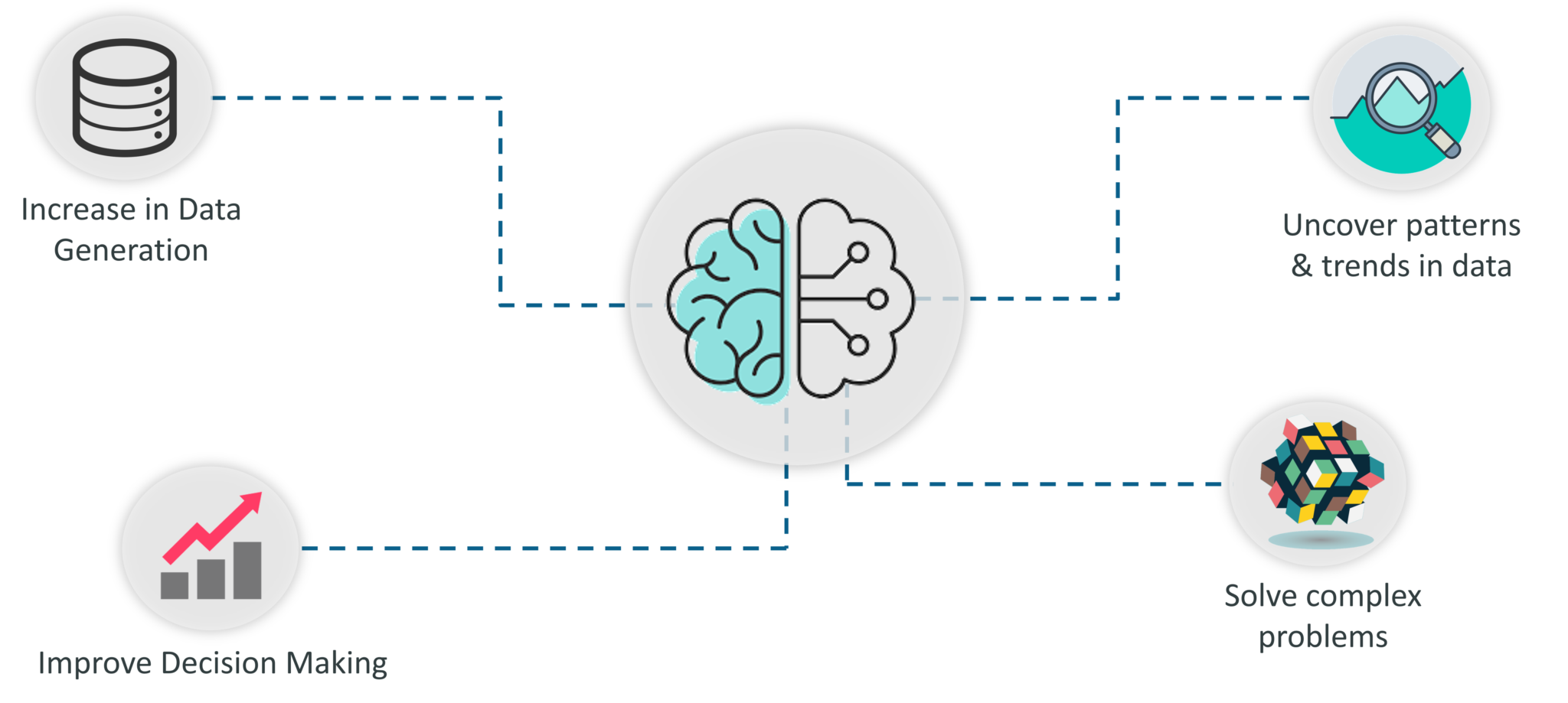
Importance Of Machine Learning – Introduction To Machine Learning – Edureka

• Uncover patterns & trends in data: Finding hidden patterns and extracting key insights from data is the most essential part of Machine Learning. By building predictive models and using statistical techniques, Machine Learning allows you to dig beneath the surface and explore the data at a minute scale. Understanding data and extracting patterns manually will take days, whereas Machine Learning algorithms can perform such computations in less than a second.
• Solve complex problems: From detecting the genes linked to the deadly ALS disease to building self-driving cars, Machine Learning can be used to solve the most complex problems.

To give you a better understanding of how important Machine Learning is, let’s list down a couple of Machine Learning Applications:

• Netflix’s Recommendation Engine: The core of Netflix is its infamous recommendation engine. Over 75% of what you watch is recommended by Netflix and these recommendations are made by implementing Machine Learning.
• Facebook’s Auto-tagging feature: The logic behind Facebook’s DeepMind face verification system is Machine Learning and Neural Networks. DeepMind studies the facial features in an image to tag your friends and family.
• Amazon’s Alexa: The infamous Alexa, which is based on Natural Language Processing and Machine Learning is an advanced level Virtual Assistant that does more than just play songs on your playlist. It can book you an Uber, connect with the other IoT devices at home, track your health, etc.
• Google’s Spam Filter: Gmail makes use of Machine Learning to filter out spam messages. It uses Machine Learning algorithms and Natural Language Processing to analyze emails in real-time and classify them as either spam or non-spam.

These were a few examples of how Machine Learning is implemented in Top Tier companies. Here’s a blog on the Top 10 Applications of Machine Learning, do give it a read to learn more.

Now that you know why Machine Learning is so important, let’s look at what exactly Machine Learning is.

Introduction To Machine Learning

The term Machine Learning was first coined by Arthur Samuel in the year 1959. Looking back, that year was probably the most significant in terms of technological advancements.

If you browse through the net about ‘what is Machine Learning’, you’ll get at least 100 different definitions. However, the very first formal definition was given by Tom M. Mitchell:

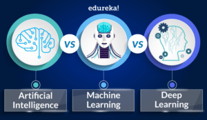
In simple terms, Machine learning is a subset of Artificial Intelligence (AI) which provides machines the ability to learn automatically & improve from experience without being explicitly programmed to do so. In the sense, it is the practice of getting Machines to solve problems by gaining the ability to think.

But wait, can a machine think or make decisions? Well, if you feed a machine a good amount of data, it will learn how to interpret, process and analyze this data by using Machine Learning Algorithms, in order to solve real-world problems.

Before moving any further, let’s discuss some of the most commonly used terminologies in Machine Learning.

Machine Learning Definitions

Algorithm: A Machine Learning algorithm is a set of rules and statistical techniques used to learn patterns from data and draw significant information from it. It is the logic behind a Machine Learning model. An example of a Machine Learning algorithm is the Linear Regression algorithm.

Model: A model is the main component of Machine Learning. A model is trained by using a Machine Learning Algorithm. An algorithm maps all the decisions that a model is supposed to take based on the given input, in order to get the correct output.

Predictor Variable: It is a feature(s) of the data that can be used to predict the output.

Response Variable: It is the feature or the output variable that needs to be predicted by using the predictor variable(s).

Training Data: The Machine Learning model is built using the training data. The training data helps the model to identify key trends and patterns essential to predict the output.

Testing Data: After the model is trained, it must be tested to evaluate how accurately it can predict an outcome. This is done by the testing data set.

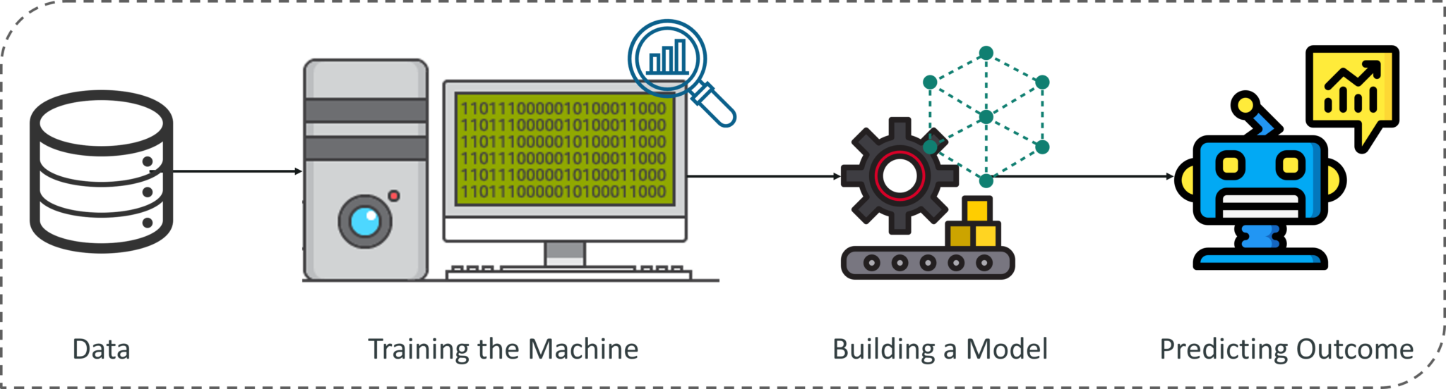
What Is Machine Learning? – Introduction To Machine Learning – Edureka

To sum it up, take a look at the above figure. A Machine Learning process begins by feeding the machine lots of data, by using this data the machine is trained to detect hidden insights and trends. These insights are then used to build a Machine Learning Model by using an algorithm in order to solve a problem.

The next topic in this Introduction to Machine Learning blog is the Machine Learning Process.

Machine Learning Process

The Machine Learning process involves building a Predictive model that can be used to find a solution for a Problem Statement. To understand the Machine Learning process let’s assume that you have been given a problem that needs to be solved by using Machine Learning.

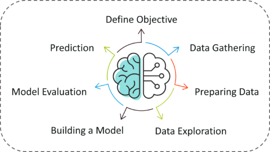
Machine Learning Process – Introduction To Machine Learning – Edureka

The problem is to predict the occurrence of rain in your local area by using Machine Learning.

The below steps are followed in a Machine Learning process:

Step 1: Define the objective of the Problem Statement

At this step, we must understand what exactly needs to be predicted. In our case, the objective is to predict the possibility of rain by studying weather conditions. At this stage, it is also essential to take mental notes on what kind of data can be used to solve this problem or the type of approach you must follow to get to the solution.

Step 2: Data Gathering

At this stage, you must be asking questions such as,

• What kind of data is needed to solve this problem?
• Is the data available?
• How can I get the data?

Once you know the types of data that is required, you must understand how you can derive this data. Data collection can be done manually or by web scraping. However, if you’re a beginner and you’re just looking to learn Machine Learning you don’t have to worry about getting the data. There are 1000s of data resources on the web, you can just download the data set and get going.

Coming back to the problem at hand, the data needed for weather forecasting includes measures such as humidity level, temperature, pressure, locality, whether or not you live in a hill station, etc. Such data must be collected and stored for analysis.

Step 3: Data Preparation

The data you collected is almost never in the right format. You will encounter a lot of inconsistencies in the data set such as missing values, redundant variables, duplicate values, etc. Removing such inconsistencies is very essential because they might lead to wrongful computations and predictions. Therefore, at this stage, you scan the data set for any inconsistencies and you fix them then and there.

Step 4: Exploratory Data Analysis

Grab your detective glasses because this stage is all about diving deep into data and finding all the hidden data mysteries. EDA or Exploratory Data Analysis is the brainstorming stage of Machine Learning. Data Exploration involves understanding the patterns and trends in the data. At this stage, all the useful insights are drawn and correlations between the variables are understood.

For example, in the case of predicting rainfall, we know that there is a strong possibility of rain if the temperature has fallen low. Such correlations must be understood and mapped at this stage.

Step 5: Building a Machine Learning Model

All the insights and patterns derived during Data Exploration are used to build the Machine Learning Model. This stage always begins by splitting the data set into two parts, training data, and testing data. The training data will be used to build and analyze the model. The logic of the model is based on the Machine Learning Algorithm that is being implemented.

In the case of predicting rainfall, since the output will be in the form of True (if it will rain tomorrow) or False (no rain tomorrow), we can use a Classification Algorithm such as Logistic Regression.

Choosing the right algorithm depends on the type of problem you’re trying to solve, the data set and the level of complexity of the problem. In the upcoming sections, we will discuss the different types of problems that can be solved by using Machine Learning.

Step 6: Model Evaluation & Optimization

After building a model by using the training data set, it is finally time to put the model to a test. The testing data set is used to check the efficiency of the model and how accurately it can predict the outcome. Once the accuracy is calculated, any further improvements in the model can be implemented at this stage. Methods like parameter tuning and cross-validation can be used to improve the performance of the model.

Step 7: Predictions

Once the model is evaluated and improved, it is finally used to make predictions. The final output can be a Categorical variable (eg. True or False) or it can be a Continuous Quantity (eg. the predicted value of a stock).

In our case, for predicting the occurrence of rainfall, the output will be a categorical variable.

So that was the entire Machine Learning process. Now it’s time to learn about the different ways in which Machines can learn.

Machine Learning Types

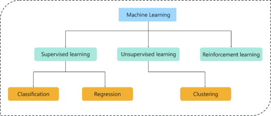
A machine can learn to solve a problem by following any one of the following three approaches. These are the ways in which a machine can learn:

1. Supervised Learning
2. Unsupervised Learning
3. Reinforcement Learning

Supervised Learning

To understand Supervised Learning let’s consider an analogy. As kids we all needed guidance to solve math problems. Our teachers helped us understand what addition is and how it is done. Similarly, you can think of supervised learning as a type of Machine Learning that involves a guide. The labeled data set is the teacher that will train you to understand patterns in the data. The labeled data set is nothing but the training data set.

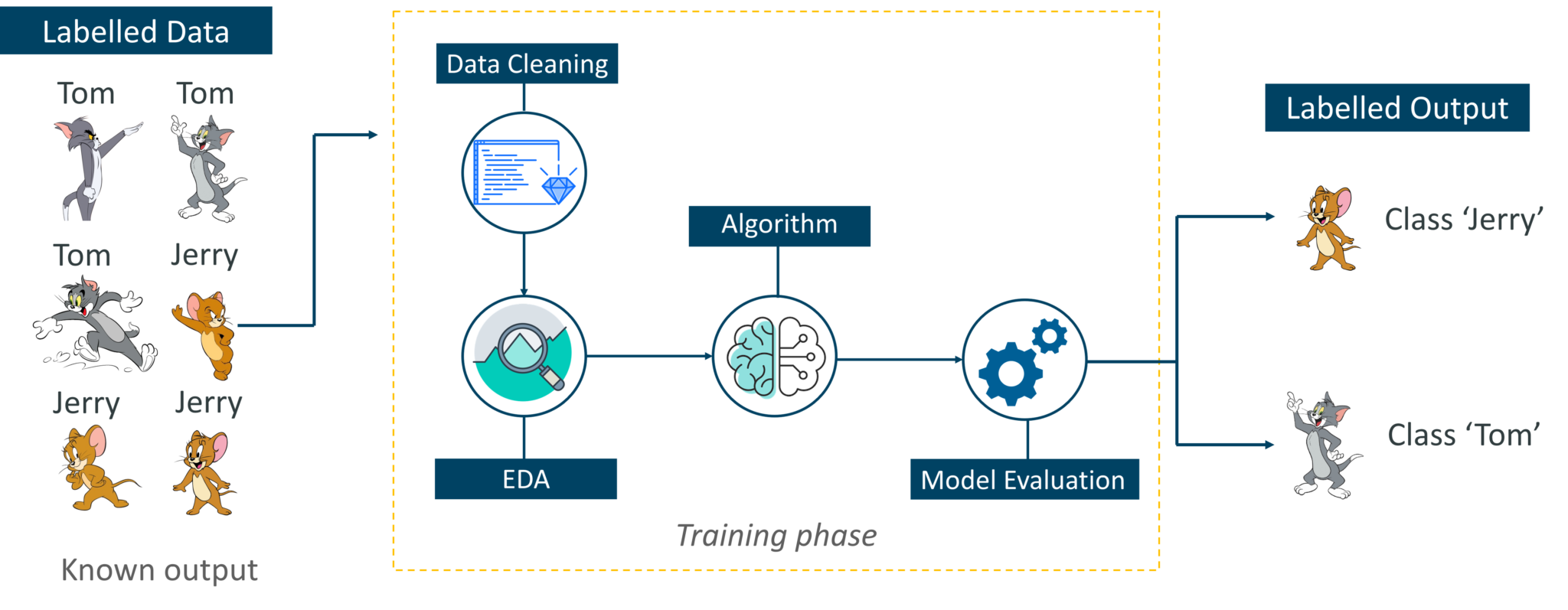
Supervised Learning – Introduction To Machine Learning – Edureka

Consider the above figure. Here we’re feeding the machine images of Tom and Jerry and the goal is for the machine to identify and classify the images into two groups (Tom images and Jerry images). The training data set that is fed to the model is labeled, as in, we’re telling the machine, ‘this is how Tom looks and this is Jerry’. By doing so you’re training the machine by using labeled data. In Supervised Learning, there is a well-defined training phase done with the help of labeled data.

Unsupervised Learning

Think of unsupervised learning as a smart kid that learns without any guidance. In this type of Machine Learning, the model is not fed with labeled data, as in the model has no clue that ‘this image is Tom and this is Jerry’, it figures out patterns and the differences between Tom and Jerry on its own by taking in tons of data.

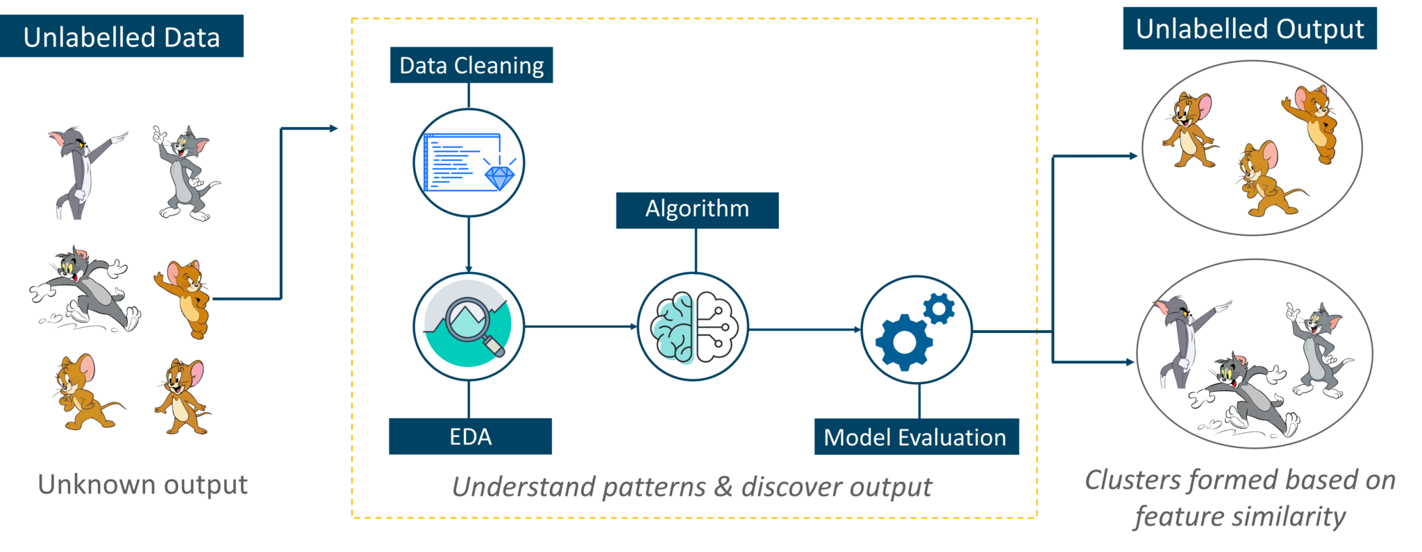
Unsupervised Learning – Introduction To Machine Learning – Edureka

For example, it identifies prominent features of Tom such as pointy ears, bigger size, etc, to understand that this image is of type 1. Similarly, it finds such features in Jerry and knows that this image is of type 2. Therefore, it classifies the images into two different classes without knowing who Tom is or Jerry is.

Reinforcement Learning

Panic? Yes, of course, initially we all would. But as time passes by, you will learn how to live on the island. You will explore the environment, understand the climate condition, the type of food that grows there, the dangers of the island, etc. This is exactly how Reinforcement Learning works, it involves an Agent (you, stuck on the island) that is put in an unknown environment (island), where he must learn by observing and performing actions that result in rewards.

Reinforcement Learning is mainly used in advanced Machine Learning areas such as self-driving cars, AplhaGo, etc.

To better understand the difference between Supervised, Unsupervised and Reinforcement Learning, you can go through this short video.

So that sums up the types of Machine Learning. Now, let’s look at the type of problems that are solved by using Machine Learning.

Type Of Problems In Machine Learning

Type of Problems Solved Using Machine Learning – Introduction To Machine Learning – Edureka

Consider the above figure, there are three main types of problems that can be solved in Machine Learning:

1. Regression: In this type of problem the output is a continuous quantity. So, for example, if you want to predict the speed of a car given the distance, it is a Regression problem. Regression problems can be solved by using Supervised Learning algorithms like Linear Regression.
2. Classification: In this type, the output is a categorical value. Classifying emails into two classes, spam and non-spam is a classification problem that can be solved by using Supervised Learning classification algorithms such as Support Vector Machines, Naive Bayes, Logistic Regression, K Nearest Neighbor, etc.
3. Clustering: This type of problem involves assigning the input into two or more clusters based on feature similarity. For example, clustering viewers into similar groups based on their interests, age, geography, etc can be done by using Unsupervised Learning algorithms like K-Means Clustering.

Here’s a table that sums up the difference between Regression, Classification, and Clustering.

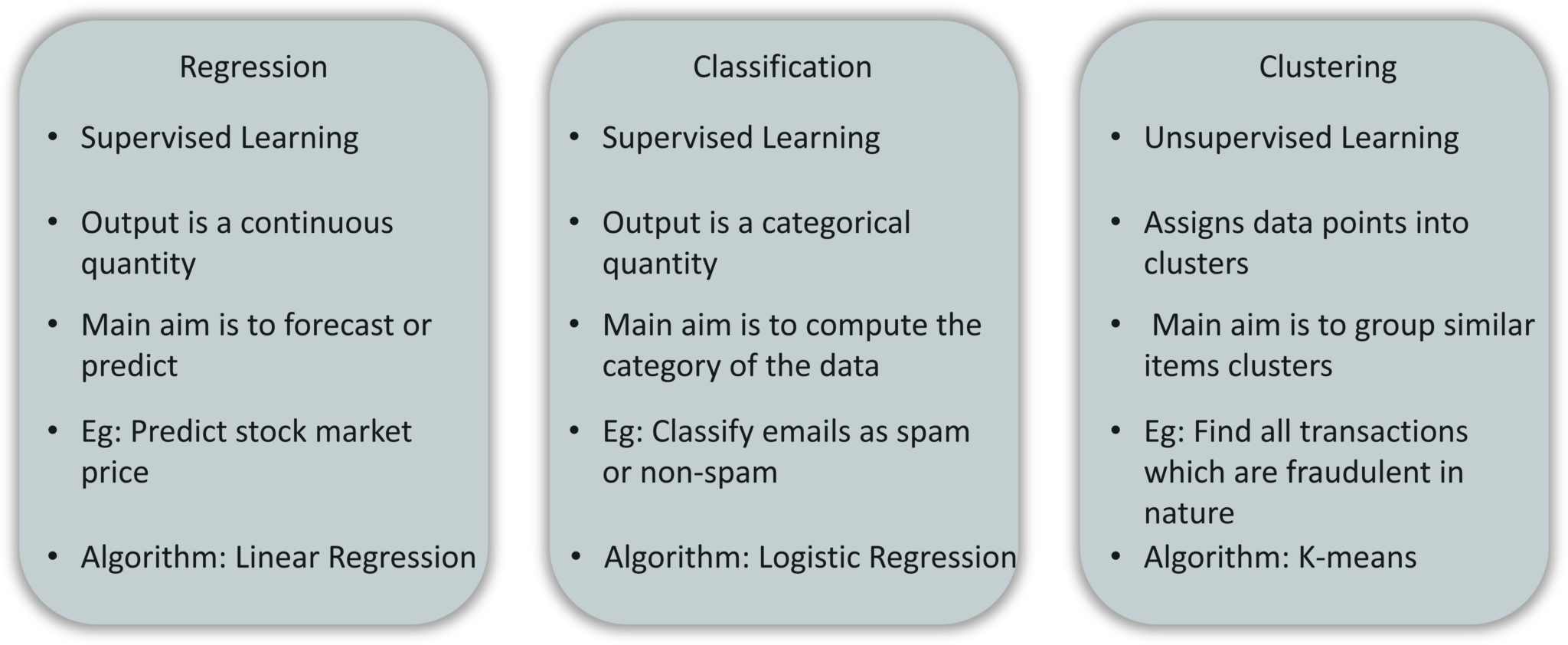
Regression vs Classification vs Clustering – Introduction To Machine Learning – Edureka

Now to make things interesting, I will leave a couple of problem statements below and your homework is to guess what type of problem (Regression, Classification or Clustering) it is:

1. Problem Statement 1: Study a bank credit dataset and make a decision about whether to approve the loan of an applicant based on his socio-economic profile.
2. Problem Statement 2: To study the House Sales dataset and build a Machine Learning model that predicts the house pricing index.
3. Problem Statement 3: To cluster a set of movies as either good or average based on their social media outreach.

Don’t forget to leave your answer in the comment section.

Now that you have a good idea about what Machine Learning is and the processes involved in it, let’s execute a demo that will help you understand how Machine Learning really works.

Machine Learning In R

A short disclaimer: I’ll be using the R language to show how Machine Learning works. R is a Statistical programming language mainly used for Data Science and Machine Learning. To learn more about R, you can go through the following blogs:

1. R Tutorial – A Beginner’s Guide to Learn R Programming
2. R Programming – Beginners Guide To R Programming Language
3. Top 50 R Interview Questions You Must Prepare in 2019
4. A Comprehensive Guide To R For Data Science

Now, let’s get started.

Problem Statement: To study the Seattle Weather Forecast Data set and build a Machine Learning model that can predict the possibility of rain.

Data Set Description: The data set was gathered by researching and observing the weather conditions at the Seattle-Tacoma International Airport. The dataset contains the following variables:

• DATE = date of the observation
• PRCP = amount of precipitation, in inches
• TMAX = maximum temperature for that day, in degrees Fahrenheit
• TMIN = minimum temperature for that day, in degrees Fahrenheit
• RAIN = TRUE if rain was observed on that day, FALSE if it was not

The target or the response variable, in this case, is ‘RAIN’. If you notice, this variable is categorical in nature, i.e. it’s value is of two categories, either True or False. Therefore, this is a classification problem and we will be using a classification algorithm called Logistic Regression.

Even though the name suggests that it is a ‘Regression’ algorithm, it actually isn’t. It belongs to the GLM (Generalised Linear Model) family and thus the name Logistic Regression.

Follow this, Comprehensive Guide To Logistic Regression In R blog to learn more about Logistic Regression.

Logic: To build a Logistic Regression model in order to predict whether or not it will rain on a particular day based on the weather conditions.

Now that you know the objective of this demo, let’s get our brains working and start coding.

Step 1: Install and load libraries

R provides 1000s of packages to run Machine Learning algorithms and mathematical models. So the first step is to install and load all the relevant libraries.

#Load required libraries
library(tidyverse)
library(boot)
install.packages('forecast')
library(forecast)
library(tseries)
install.packages('caret')
library(caret)
install.packages('ROCR')
library(ROCR)

Each of these libraries serves a specific purpose, you can read more about the libraries in the official R Documentation.

Step 2: Import the Data set

Lucky for me I found the data set online and so I don’t have to manually collect it. In the below code snippet, I’ve loaded the data set into a variable called ‘data.df’ by using the ‘read.csv()’ function provided by R. This function is to load a Comma Separated Version (CSV) file.

#Import data set
data.df <- read.csv("/Users/Zulaikha_Geer/Desktop/Data/seattleWeather_1948-2017.csv", header = TRUE)

Step 3: Studying the Data Set

Let’s take a look at a couple of observations in the data set. To do this we can use the head() function provided by R. This will list down the first 6 observations in the data set.

> head(data.df)
DATE     PRCP   TMAX   TMIN  RAIN
1 1948-01-01    0.47       51      42    TRUE
2 1948-01-02   0.59      45      36    TRUE
3 1948-01-03   0.42      45      35    TRUE
4 1948-01-04   0.31      45      34     TRUE
5 1948-01-05   0.17      45      32     TRUE
6 1948-01-06   0.44     48      39     TRUE

Now, let’s look at the structure if the data set by using the str() function.

#Studying the structure of the data set
> str(data.df)
'data.frame': 25551 obs. of 5 variables:
$ DATE: Factor w/ 25551 levels "1948-01-01","1948-01-02",..: 1 2 3 4 5 6 7 8 9 10 ...
$ PRCP: num 0.47 0.59 0.42 0.31 0.17 0.44 0.41 0.04 0.12 0.74 ...
$ TMAX: int 51 45 45 45 45 48 50 48 50 43 ...
$ TMIN: int 42 36 35 34 32 39 40 35 31 34 ...
$ RAIN: logi TRUE TRUE TRUE TRUE TRUE TRUE ...

In the above code, you can see that the data type for the ‘DATE’ and ‘RAIN’ variable is not correctly formatted. The ‘DATE’ variable must be of type Date and the ‘RAIN’ variable must be a factor.

Step 4: Data Cleaning

The below code snippet while format the ‘DATE’ and ‘RAIN’ variable:

#Formatting 'date' and 'rain' variable
data.df$DATE <- as.Date(data.df$DATE)
data.df$RAIN <- as.factor(data.df$RAIN)

Like I mentioned earlier, it is essential to check for any missing or NA values in the data set, the below code snippet checks for NA values in each variable:

#Checking for NA values in the 'DATE' variable
> which(is.na(data.df$DATE))
integer(0)

#Checking for NA values in the 'TMAX' variable
> which(is.na(data.df$TMAX))
integer(0)

#Checking for NA values in the 'TMIN' variable
> which(is.na(data.df$TMIN))
integer(0)

#Checking for NA values in the 'PRCP' variable
> which(is.na(data.df$PRCP))
[1] 18416 18417 21068

#Checking for NA values in the 'rain' variable
> which(is.na(data.df$RAIN))
[1] 18416 18417 21068

If you notice the above code snippet, you can see that variables, TMAX, TMIN and, DATE have no NA values, whereas the ‘PRCP’ and ‘RAIN’ variable has 3 missing values, these values must be removed.

# Remove the rows with missing RAIN value
> data.df <- data.df[-c(18416, 18417, 21068),]

The values are removed successfully!

Step 5: Data Splicing

Data Splicing is just another fancy term for splitting the data set into training and testing set. The training data set must be bigger since training the model and helping it study the trends, requires a lot more data. The below code snippet splits the data set into training and testing sets in the ratio 7:3. Which implies that 70% of the data is used for training, whereas 30% is used for testing.

#Data Splicing
#Data Partitioning: create a train and test dataset (0.7: 0.3)
index <- createDataPartition(data.df$RAIN, p = 0.7, list = FALSE)
# Training set
train.df <- data.df[index,]
# Testing dataset
test.df <- data.df[-index,]

You can check out the summary of the testing and training data set by using the summary() function in R:

> summary(train.df)

> summary(test.df)

Step 6: Data Exploration

This stage involves detecting patterns in the data and finding out correlations between predictor variables and the response variable. In the below code snippet I’ve used the cor.test() function provided by R.

This correlation test shows the significance of the predictor variables in building the model. Also, the cor.test() function requires you to have variables of type numeric, that’s why in the below code I’ve formatted the ‘Rain’ variable as numeric.

#Setting rain variable as numeric for computing the correlation
train.df$RAIN <- as.numeric(train.df$RAIN) #Correlation between 'Rain' variable and 'TMAX' > cor.test(train.df$TMAX, train.df$RAIN)

Pearson's product-moment correlation

data: train.df$TMAX and train.df$RAIN
t = -55.492, df = 17882, p-value < 2.2e-16 alternative hypothesis: true correlation is not equal to 0 95 percent confidence interval: -0.3957173 -0.3707104 sample estimates: cor -0.3832841 > #Correlation between 'Rain' variable and 'TMIN'
cor.test(train.df$TMIN, train.df$RAIN)

Pearson's product-moment correlation

data: train.df$TMIN and train.df$RAIN
t = -18.163, df = 17882, p-value < 2.2e-16
alternative hypothesis: true correlation is not equal to 0
95 percent confidence interval:
-0.1489493 -0.1201678
sample estimates:
cor
-0.1345869

The above output shows that both TMIN and TMAX are significant predictor variables. Notice the p-value for both the variables. The p-value or the probability value is the most essential parameter to understand the significance of a model.

If the p-value of a variable is less than 0.05 it is considered to be an important feature in predicting the outcome. In our case, the p-value for each of these variables is way below 0.05 which is a good thing.

Before moving further let’s convert the ‘RAIN’ variable back into the ‘factor’ type:

#Setting rain variable as a factor for building the model
train.df$RAIN <- as.factor(train.df$RAIN)

Step 7: Building a Machine Learning model

After understanding the correlations, it’s time to build the model. We’ll be using the Logistic Regression algorithm to build the model. R provides a function called glm() that contains the Logistic Regression algorithm. The syntax for the glm() function is:

glm(formula, data, family)

In the above syntax:

• Formula: The formula represents the relationship between the dependent and independent variables.
• Data: The data set on which the formula is applied.
• Family: This field specifies the type of regression model. In our case, it is a binary logistic regression model.

> #Building a Logictic regression model
> # glm logistic regression
> model <- glm(RAIN ~ TMAX + TMIN, data = train.df, family = binomial) > summary(model)

Call:
glm(formula = RAIN ~ TMAX + TMIN, family = binomial, data = train.df)

Deviance Residuals:
Min 1Q Median 3Q Max
-2.4700 -0.8119 -0.2557 0.8490 3.2691

Coefficients:
Estimate Std. Error z value Pr(>|z|)
(Intercept) 2.808373 0.098668 28.46 <2e-16 ***
TMAX -0.250859 0.004121 -60.87 <2e-16 ***
TMIN 0.259747 0.005036 51.57 <2e-16 ***
---
Signif. codes: 0 &lsquo;***&rsquo; 0.001 &lsquo;**&rsquo; 0.01 &lsquo;*&rsquo; 0.05 &lsquo;.&rsquo; 0.1 &lsquo; &rsquo; 1

(Dispersion parameter for binomial family taken to be 1)

Null deviance: 24406 on 17883 degrees of freedom
Residual deviance: 17905 on 17881 degrees of freedom
AIC: 17911

Number of Fisher Scoring iterations: 5

We’ve successfully built the model by using the ‘TMAX’ and ‘TMIN’ variables since they have a strong correlation with the target variable (‘Rain’).

Step 8: Model Evaluation

At this step, we’re going to validate the efficiency of the Machine Learning model by using the testing data set.

#Model Evaluation
#Storing predicted values
> predicted_values <- predict(model, test.df, type = "response") > head(predicted_values)
2 4 5 8 9 18
0.7048729 0.5868884 0.4580049 0.4646309 0.1567753 0.8585068

#Creating a table containing the actual 'RAIN' values in the test data set
> table(test.df$RAIN)

FALSE TRUE
4394&nbsp; &nbsp; &nbsp;3270
> nrows_prediction<-nrow(test.df) #Creating a data frame containing the predicted 'Rain' values > prediction <- data.frame(c(1:nrows_prediction)) > colnames(prediction) <- c("RAIN") > str(prediction)
'data.frame': 7664 obs. of 1 variable:
$ RAIN: int 1 2 3 4 5 6 7 8 9 10 ...

#Converting the 'Rain' variable into a character that stores either (T/F)
prediction$RAIN <- as.character(prediction$RAIN)

#Setting the threshold value
prediction$RAIN <- "TRUE"
prediction$RAIN[ predicted_values < 0.5] <- "FALSE" #prediction [predicted_values > 0.5] <- "TRUE"
prediction$RAIN <- as.factor(prediction$RAIN)

Refer the comments for the code, it is easily understandable.

#Comparing the predicted values and the actual values
> table(prediction$RAIN, test.df$RAIN)

FALSE TRUE
FALSE    3460    931
TRUE       934    2339

In the below code snippet we’re using the Confusion matrix to evaluate the accuracy of the model.

#Confusion Matrix
> confusionMatrix(prediction$RAIN, test.df$RAIN)
Confusion Matrix and Statistics

Reference
Prediction FALSE TRUE
FALSE 3460 931
TRUE 934 2339

Accuracy : 0.7567
95% CI : (0.7469, 0.7662)
No Information Rate : 0.5733
P-Value [Acc > NIR] : <2e-16

Kappa : 0.5027

Mcnemar's Test P-Value : 0.9631

Sensitivity : 0.7874
Specificity : 0.7153
Pos Pred Value : 0.7880
Neg Pred Value : 0.7146
Prevalence : 0.5733
Detection Rate : 0.4515
Detection Prevalence : 0.5729
Balanced Accuracy : 0.7514

'Positive' Class : FALSE

As per the above output, the model can predict the possibility of rainfall with an accuracy of approximately 76% which is quite good. To sum it up, let’s plot a graph that shows the Logistic Regression curve, which is known as the Sigmoid curve between the predictor variable TMAX and the target variable RAIN.

#Output plot showing the variation between TMAX and Rainfall
ggplot(test.df, aes(x = test.df$TMAX, y = predicted_values))+
geom_point() + # add points
geom_smooth(method = "glm", # plot a regression...
method.args = list(family = "binomial"))

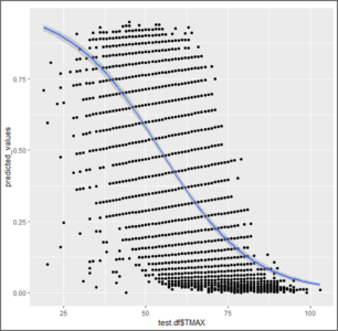
ggplot – Introduction To Machine Learning – Edureka

Now that you know Machine Learning Basics, I’m sure you’re curious to learn more about the various Machine learning algorithms. Here’s a list of blogs that cover the different types of Machine Learning algorithms in depth:

• Linear Regression
• Logistic Regression
• Support Vector Machine
• Decision Trees
• Random Forest
• Naive Bayes
• K Nearest Neighbor
• K-Means

So, with this, we come to the end of this Introduction To Machine Learning blog. I hope you all found this blog informative and if not then you can also join our Machine Learning certification at Edureka. If you have any thoughts to share, please comment them below. Stay tuned for more blogs like these!