
Data Science with Python Certification Course
- 132k Enrolled Learners
- Weekend
- Live Class
(49300)


 Copy Link!
R for Data Science is a must learn for Data Analysis & Data Science professionals. With its growth in the IT industry, there is a booming demand for skilled Data Scientists who have an understanding of the major concepts in R. One such concept, is the Decision Tree.
In this blog we will discuss :
1. How to create a decision tree for the admission data.
2. Use rattle to plot the tree.
3. Validation of decision tree using the ‘Complexity Parameter’ and cross validated error.
4. Prune the tree on the basis of these parameters to create an optimal decision tree.
To understand what are decision trees and what is the statistical mechanism behind them, you can read this post : How To Create A Perfect Decision Tree
To create a decision tree in R, we need to make use of the functions rpart(), or tree(), party(), etc.
rpart() package is used to create the tree. It allows us to grow the whole tree using all the attributes present in the data.
> library("rpart")
> setwd("D://Data")
> data <- read.csv("Gre_Coll_Adm.csv")
> str(data)
 'data.frame': 400 obs. of 5 variables:
 $ X : int 1 2 3 4 5 6 7 8 9 10 ...
 $ Admission_YN : int 0 1 1 1 0 1 1 0 1 0 ...
 $ Grad_Rec_Exam: int 380 660 800 640 520 760 560 400 540 700 ...
 $ Grad_Per : num 3.61 3.67 4 3.19 2.93 3 2.98 3.08 3.39 3.92 ...
 $ Rank_of_col : int 3 3 1 4 4 2 1 2 3 2 ...
> View(data)
> adm_data<-as.data.frame(data)
> tree <- rpart(Admission_YN ~ adm_data$Grad_Rec_Exam + adm_data$Grad_Per+ adm_data$Rank_of_col,
 + data=adm_data,
 + method="class")
rpart syntax takes ‘dependent attribute’ and the rest of the attributes are independent in the analysis.
Admission_YN : Dependent Attribute. As admission depends on the factors score, rank of college, etc.
Grad_Rec_Exam, Grad_Per, and Rank_of_col : Independent Attributes
rpart() returns a Decison tree created for the data.
If you plot this tree, you can see that it is not visible, due to the limitations of the plot window in the R console.
> plot(tree)
> text(tree, pretty=0)

Let us try to fix it:

To enhance it, let us take some help from rattle :
> library(rattle)
> rattle()

Rattle() is one unique feature of R which is specifically built for data mining in R. It provides its own GUI apart from the R Console which makes it easier to analyze data. It has built-in graphics, which provides us better visualizations as well. Here we will use just the plotting capabilities of Rattle to achieve a decent decision tree plot.
> library(rpart.plot)
> library(RColorBrewer)
rpart.plot() and RcolorBrewer() functions help us to create a beautiful plot. ‘rpart.plot()’ plots rpart models. It extends plot.rpart and text.rpart in the rpart package. RcolorBrewer() provides us with beautiful color palettes and graphics for the plots.
> fancyRpartPlot(tree)

This was a simple and efficient way to create a Decision Tree in R. But are you sure that this is the optimal ‘Decision Tree’ for this data? If not, the following validation checks will help you.
Meanwhile, if you wish to learn R programming, check out our specially curated course by clicking on the below button.
To validate the model we use the printcp and plotcp functions. ‘CP’ stands for Complexity Parameter of the tree.
Syntax : printcp ( x ) where x is the rpart object.
This function provides the optimal prunings based on the cp value.
We prune the tree to avoid any overfitting of the data. The convention is to have a small tree and the one with least cross validated error given by printcp() function i.e. ‘xerror’.
Cross Validated Error :

To find out how the tree performs, is calculated by the printcp() function, based on which we can go ahead and prune the tree.
> printcp(tree)
Classification tree:
 rpart(formula = Admission_YN ~ adm_data$Grad_Rec_Exam + adm_data$Grad_Per +
 adm_data$Rank_of_col, data = adm_data, method = "class")
Variables actually used in tree construction:
 [1] adm_data$Grad_Per adm_data$Grad_Rec_Exam adm_data$Rank_of_col
Root node error: 127/400 = 0.3175
n= 400
CP nsplit rel error xerror xstd
 1 0.062992 0 1.00000 1.00000 0.073308
 2 0.023622 2 0.87402 0.92913 0.071818
 3 0.015748 4 0.82677 0.99213 0.073152
 4 0.010000 8 0.76378 1.02362 0.073760
From the above mentioned list of cp values, we can select the one having the least cross-validated error and use it to prune the tree.
The value of cp should be least, so that the cross-validated error rate is minimum.
To select this, you can make use of this :
fit$cptable[which.min(fit$cptable[,”xerror”]),”CP”]
This function returns the optimal cp value associated with the minimum error.
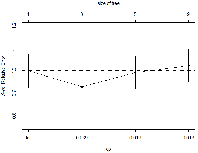
Let us see what plotcp() function fetches.
> plotcp(tree)

Plotcp() provides a graphical representation to the cross validated error summary. The cp values are plotted against the geometric mean to depict the deviation until the minimum value is reached.
> ptree<- prune(tree,
 + cp= tree$cptable[which.min(tree$cptable[,"xerror"]),"CP"])
> fancyRpartPlot(ptree, uniform=TRUE,
 + main="Pruned Classification Tree")

Thus we create a pruned decision tree.
If you wish to get a head-start on R programming, check out the Data Analytics with R course from Edureka.
Got a question for us? Please mention them in the comments section and we will get back to you.
Related Posts:


 Thank you for registering Join Edureka Meetup community for 100+ Free Webinars each month JOIN MEETUP GROUP
please send me the code
Hey Jaswant, sure. Mention your email address and we will send it over. Cheers :)
in decision tree how to find the time independent attribute and dependent attirbute
@EdurekaSupport:disqus Hi, could you please share your dataset with birukovanbn@gmail.com Thank you!
Sure @natalliabirukova:disqus we have shared the dataset with you. Do let us know if you need anything else. Cheers :)
@EdurekaSupport Hi, can you please share your dataset with burukovanbn@gmail.com
can u please share the dataset to innovationmiracleviz@gmail.com
Sure Pushpa! Thank you for watching our videos. We have shared the data set with you. Do subscribe, like and share our videos. Also, check out our website to know more about the courses we offer : https://www.edureka.co/data-science-r-programming-certification-course .
Hope this helps. Cheers :)
#rm(list=ls(all=TRUE))
setwd(“C:\Users\hp\Desktop\R”)
version
#Reading from a CSV file
univ=read.table(‘dataDemographics.csv’,
header=T,sep=’,’,
col.names=c(“ID”, “age”, “exp”, “inc”,
“zip”, “family”,
“edu”, “mortgage”))
dim(univ)
head(univ)
str(univ)
names(univ)
sum(is.na(univ))
sum(is.na(univ[[2]])) #see missig values in col 2
sapply(univ, function(x) sum(is.na(x)))
row.names.data.frame(is.na(univ))
# Reading Second Table
loanCalls <- read.table("dataLoanCalls.csv", header=T, sep=",",
col.names=c("ID", "infoReq", "loan"),
dec=".", na.strings="NA")
head(loanCalls)
dim(loanCalls)
sum(is.na(loanCalls))
sapply(loanCalls, function(x) sum(is.na(x)))
# Reading third Table
cc <- read.table("dataCC.csv", header=T, sep=",",
col.names=c("ID", "Month", "Monthly"),
dec=".", na.strings="NA")
head(cc)
dim(cc)
sum(is.na(cc))
sapply(cc, function(x)sum(is.na(x)))
#We have the monthly credit card spending over 12 months.
#We need to compute monthly spendings
tapply
head(cc)
summary(cc)
str(cc)
cc$ID <- as.factor(cc$ID)
cc$Month <- as.factor(cc$Month)
sapply(cc,function(x) length(unique(x)))
summary(cc)
# function to cal. mean
meanNA <- function(x){
a <-mean(x, na.rm=TRUE)
return(a)
}
ccAvg <- data.frame(seq(1,5000),
tapply(cc$Monthly, cc$ID, meanNA))
ccAvg
head(ccAvg)
dim(ccAvg)
names(ccAvg)
colnames(ccAvg) <- c("ID", "ccavg")
str(ccAvg)
ccAvg$ID <- as.factor(ccAvg$ID)
summary(ccAvg)
str(ccAvg)
rm(cc)
# Reading fourth table
otherAccts <- read.table("dataOtherAccts.csv", header=T, sep=",",
col.names=c("ID", "Var", "Val"),
dec=".", na.strings="NA")
dim(otherAccts)
head(otherAccts)
summary(otherAccts)
otherAccts$ID <- as.factor(otherAccts$ID)
otherAccts$Val <- as.factor(otherAccts$Val)
summary(otherAccts)
str(otherAccts)
# to transpose
library(reshape)
otherAcctsT=data.frame(cast(otherAccts,
ID~Var,value="Val"))
head(otherAcctsT)
dim(otherAcctsT)
#Merging the tables
univComp <- merge(univ,ccAvg,
by.x="ID",by.y="ID",
all=TRUE) #Outer join
univComp <- merge(univComp, otherAcctsT,
by.x="ID", by.y="ID",
all=TRUE)
univComp <- merge(univComp, loanCalls,
by.x="ID", by.y="ID",
all=TRUE)
dim(univComp)
head(univComp)
str(univComp)
summary(univComp)
names(univComp)
sum(is.na(univComp))
#Dealing with missing values
#install.packages("VIM")
library(VIM)
matrixplot(univComp)
#Filling up missing values with KNNimputation
library(DMwR)
univ2 <- knnImputation(univComp,
k = 10, meth = "median")
sum(is.na(univ2))
summary(univ2)
head(univ2,10)
univ2$family <- ceiling(univ2$family)
univ2$edu <- ceiling(univ2$edu)
head(univ2,15)
str(univ2)
names(univ2)
# converting ID, Family, Edu, loan into factor
attach(univ2)
univ2$ID <- as.factor(ID)
univ2$family <- as.factor(family)
univ2$edu <- as.factor(edu)
univ2$loan <- as.factor(loan)
str(univ2)
summary(univ2)
sapply(univ2, function(x) length(unique(x)))
# removing the id, Zip and experience as experience
# is correlated to age
names(univ2)
univ2Num <- subset(univ2, select=c(2,3,4,8,9))
head(univ2Num)
cor(univ2Num)
names(univ2)
univ2 <- univ2[,-c(1,3,5)]
str(univ2)
summary(univ2)
# Converting the categorical variables into factors
# Discretizing age and income into categorial variables
library(infotheo)
#Discretizing the variable 'age'
age <- discretize(univ2$age, disc="equalfreq",
nbins=10)
class(age)
head(age)
age=as.factor(age$X)
#Discretizing the variable 'inc'
inc=discretize(univ2$inc, disc="equalfreq",
nbins=10)
head(inc)
inc=as.factor(inc$X)
#Discretizing the variable 'age'
ccavg=discretize(univ2$ccavg, disc="equalwidth",
nbins=10)
ccavg=as.factor(ccavg$X)
#Discretizing the variable 'age'
mortgage=discretize(univ2$mortgage, disc="equalwidth",
nbins=5)
mortgage=as.factor(mortgage$X)
# *** Removing the numerical variables from the original
# *** data and adding the categorical forms of them
head(univ2)
univ2 <- subset(univ2, select= -c(age,inc,ccavg,mortgage))
head(univ2)
univ2 <- cbind(age,inc,ccavg,mortgage,univ2)
head(univ2,20)
dim(univ2)
str(univ2)
summary(univ2)
# Let us divide the data into training, testing
# and evaluation data sets
rows=seq(1,5000,1)
set.seed(123)
trainRows=sample(rows,3000)
set.seed(123)
remainingRows=rows[-(trainRows)]
testRows=sample(remainingRows, 1000)
evalRows=rows[-c(trainRows,testRows)]
train = univ2[trainRows,]
test=univ2[testRows,]
eval=univ2[evalRows,]
dim(train); dim(test); dim(eval)
rm(age,ccavg, mortgage, inc, univ)
#### Building Models
#Decision Trees using C50
names(train)
#install.packages("C50")
library(C50)
dtC50 <- C5.0(loan ~ ., data = train, rules=TRUE)
summary(dtC50)
predict(dtC50, newdata=train, type="class")
a=table(train$loan, predict(dtC50,
newdata=train, type="class"))
rcTrain=(a[2,2])/(a[2,1]+a[2,2])*100
rcTrain
# Predicting on Testing Data
predict(dtC50, newdata=test, type="class")
a=table(test$loan, predict(dtC50,
newdata=test, type="class"))
rcTest=(a[2,2])/(a[2,1]+a[2,2])*100
rcTest
# Predicting on Evaluation Data
predict(dtC50, newdata=eval, type="class")
a=table(eval$loan, predict(dtC50,
newdata=eval, type="class"))
rcEval=(a[2,2])/(a[2,1]+a[2,2])*100
rcEval
cat("Recall in Training", rcTrain, 'n',
"Recall in Testing", rcTest, 'n',
"Recall in Evaluation", rcEval)
#Test by increasing the number of bins in inc and ccavg to 10
#Test by changing the bin to euqalwidth in inc and ccavg
library(ggplot2)
#using qplot
qplot(edu, inc, data=univ2, color=loan,
size=as.numeric(ccavg))+
theme_bw()+scale_size_area(max_size=9)+
xlab("Educational qualifications") +
ylab("Income") +
theme(axis.text.x=element_text(size=18),
axis.title.x = element_text(size =18,
colour = 'black'))+
theme(axis.text.y=element_text(size=18),
axis.title.y = element_text(size = 18,
colour = 'black',
angle = 90))
#using ggplot
ggplot(data=univ2,
aes(x=edu, y=inc, color=loan,
size=as.numeric(ccavg)))+
geom_point()+
scale_size_area(max_size=9)+
xlab("Educational qualifications") +
ylab("Income") +
theme_bw()+
theme(axis.text.x=element_text(size=18),
axis.title.x = element_text(size =18,
colour = 'black'))+
theme(axis.text.y=element_text(size=18),
axis.title.y = element_text(size = 18,
colour = 'black',
angle = 90))
rm(a,rcEval,rcTest,rcTrain)
#—————————————————
#Decision Trees using CART
#Load the rpart package
library(rpart)
#Use the rpart function to build a classification tree model
dtCart <- rpart(loan ~ ., data=train, method="class", cp = .001)
#Type churn.rp to retrieve the node detail of the
#classification tree
dtCart
#Use the printcp function to examine the complexity parameter
printcp(dtCart)
#use the plotcp function to plot the cost complexity parameters
plotcp(dtCart)
#plot function and the text function to plot the classification tree
plot(dtCart,main="Classification Tree for loan Class",
margin=.1, uniform=TRUE)
text(dtCart, use.n=T)
## steps to validate the prediction performance of a classification tree
————————————————————————
predict(dtCart, newdata=train, type="class")
a <- table(train$loan, predict(dtCart,
newdata=train, type="class"))
dtrain <- (a[2,2])/(a[2,1]+a[2,2])*100
a <-table(test$loan, predict(dtCart,
newdata=test, type="class"))
dtest <- (a[2,2])/(a[2,1]+a[2,2])*100
a <- table(eval$loan, predict(dtCart,
newdata=eval, type="class"))
deval <- (a[2,2])/(a[2,1]+a[2,2])*100
cat("Recall in Training", dtrain, 'n',
"Recall in Testing", dtest, 'n',
"Recall in Evaluation", deval)
#### Pruning a tree
——————–
#Finding the minimum cross-validation error of the
#classification tree model
min(dtCart$cptable[,"xerror"])
#Locate the record with the minimum cross-validation errors
which.min(dtCart$cptable[,"xerror"])
#Get the cost complexity parameter of the record with
#the minimum cross-validation errors
dtCart.cp <- dtCart$cptable[5,"CP"]
dtCart.cp
#Prune the tree by setting the cp parameter to the CP value
#of the record with minimum cross-validation errors:
prune.tree <- prune(dtCart, cp= dtCart.cp)
prune.tree
#Visualize the classification tree by using the plot and
#text function
plot(prune.tree, margin= 0.01)
text(prune.tree, all=FALSE , use.n=TRUE)
## steps to validate the prediction performance of a classification tree
————————————————————————
a <- table(train$loan, predict(prune.tree,
newdata=train, type="class"))
dtrain <- (a[2,2])/(a[2,1]+a[2,2])*100
a <-table(test$loan, predict(prune.tree,
newdata=test, type="class"))
dtest <- (a[2,2])/(a[2,1]+a[2,2])*100
a <- table(eval$loan, predict(prune.tree,
newdata=eval, type="class"))
deval <- (a[2,2])/(a[2,1]+a[2,2])*100
cat("Recall in Training", dtrain, 'n',
"Recall in Testing", dtest, 'n',
"Recall in Evaluation", deval)
#———————————————————
# Decision tree using Conditional Inference
library(party)
ctree.model= ctree(loan ~ ., data = train)
plot(ctree.model)
a=table(train$loan, predict(ctree.model, newdata=train))
djtrain <- (a[2,2])/(a[2,1]+a[2,2])*100
a=table(test$loan, predict(ctree.model, newdata=test))
djtest <- (a[2,2])/(a[2,1]+a[2,2])*100
a=table(eval$loan, predict(ctree.model, newdata=eval))
djeval <- (a[2,2])/(a[2,1]+a[2,2])*100
cat("Recall in Training", djtrain, 'n',
"Recall in Testing", djtest, 'n',
"Recall in Evaluation", djeval)
Is there a need to split the original data set into a test and training set? Or, is the testing of the model being done in the pruning/cross-validation steps? Thank you. Great blog!
please share the data set to my email id- sravanakabilvam@gmail.com @@EdurekaSupport:disqus
Well explained with complete R code!!
Could you please also provide the link to download the data sets on every topic that you had explained in this blog? that would be a great help for us!! Thank you!
Please send me the data file at thanlong281984@yahoo.com.vn