
Data Science with Python Certification Course
- 132k Enrolled Learners
- Weekend
- Live Class
(49300)


 Copy Link!
Once in every 4 years, the world celebrates a festival called “Fifa World Cup” and with that, everything seems to change. Priorities switch to football, and predictions switch to the teams and players that would perform in the tournament. Through the medium of this blog, I am going to predict the “World’s Best Playing XI” in 2018 and I would be using Python for the analytical implementation.
Analyze the Fifa Dataset to predict the World’s Best Playing XI in 2018!!
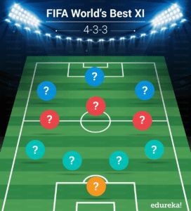
In my quest to carry out the above mentioned task, I stumbled upon an interesting dataset on Kaggle. I am going to stick with it and use it to predict the strongest 11 players taking part in this world cup 2018. Based on player availability, the best possible lineup is a 4-3-3. Using this dataset, I would be giving you a step by step approach to analyze various characteristics that would help us infer the best players for the World Cup 2018.
So, let’s get started :-)
Let’s start by importing the dataset and the required libraries in Python.
import pandas as pd
import seaborn as sns
import matplotlib.pyplot as plt
import numpy as np
% matplotlib inline
df = pd.read_csv("FullData.csv")
df.head(7)
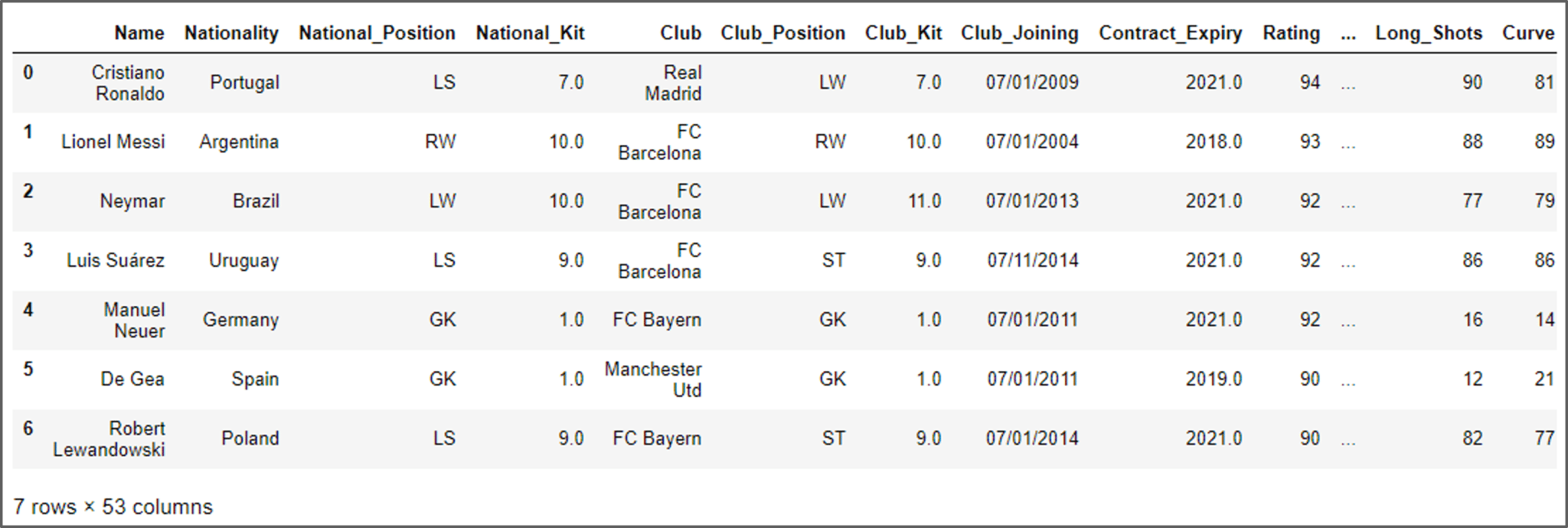
It is evident from the above screenshot, there are 53 columns which include the following attributes:
Name, Nationality, National_Position, National_Kit, Club, Club_Position, Club_Kit, Club_Joining, Contract_Expiry, Rating, Height, Weight, Preffered_Foot, Birth_Date, Age, Preffered_Position, Work_Rate, Weak_foot, Skill_Moves, Ball_Control, Dribbling, Marking, Sliding_Tackle, Standing_Tackle, Aggression, Reactions, Attacking_Position, Interceptions, Vision, Composure, Crossing, Short_Pass, Long_Pass, Acceleration, Speed, Stamina, Strength, Balance, Agility, Jumping, Heading, Shot_Power, Finishing, Long_Shots, Curve, Freekick_Accuracy, Penalties, Volleys, GK_Positioning, GK_Diving, GK_Kicking, GK_Handling and GK_Reflexes.
Analyzing this huge dataset is a tedious task as it involves quite a few pre-processing steps. There might be a lot of redundant and unwanted columns, which can be removed. Therefore you can delete certain columns if needed, by writing the below code:
del df['National_Kit'] #deletes the column National_Kit
df.head()
Once you have simplified this data, you can then start with the analysis part. Let us begin with the simplest plot. This graph gives us the number of players representing a particular country. Now, these graphs are best used to gain statistical insights.
plt.figure(figsize=(15,32))

sns.countplot(y = df.Nationality,palette="Set2") #Plot all the nations on Y Axis
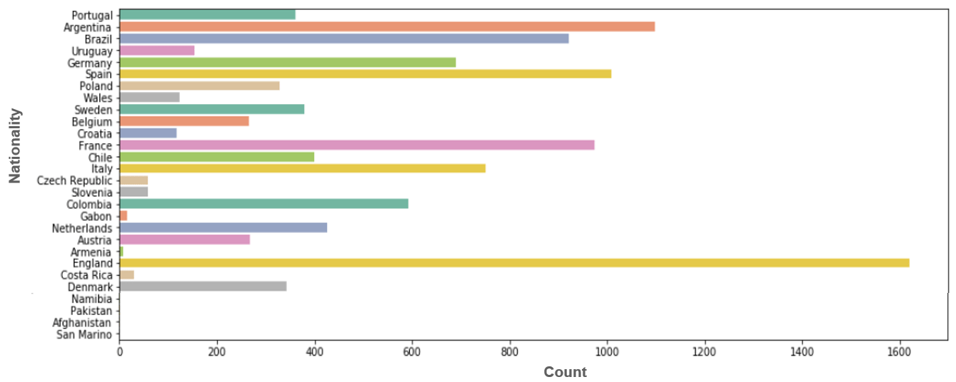
Note: The plot generated from the above code will display all the football playing nations, but for the sake of simplicity, I have just displayed the top 28 countries which would give me the desired results.
Using this graph, we conclude that most of the players are from England, Argentina, Spain, France and Brazil. In this case, the graph won’t add a lot of value because we would be picking the best XI, and the results may vary.
Moving ahead with the analysis, you can try out different visualizations with the player’s age, preferred_position, rating, club etc. Let me show you one such visualization and then we’ll switch to our analysis of the best playing XI for the world cup.
plt.figure(figsize=(15,6))
sns.countplot(x="Age",data=df)
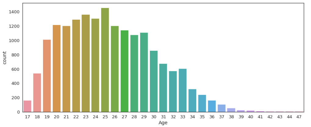
It is evident from the above screenshot that the majority of players are between the age of 20 and 29, with the largest peak of 25 years.
Now is the time we try and find the answer to the question put forth in the problem statement: Who will be the World’s Best Playing XI?
Let us begin our analysis. Let us start by considering the following playing formation, 4-3-3. So here, we need to find 4 best defenders, 3 best mid-fielders and 3 best attackers. Let us start our quest by finding a goalkeeper first.
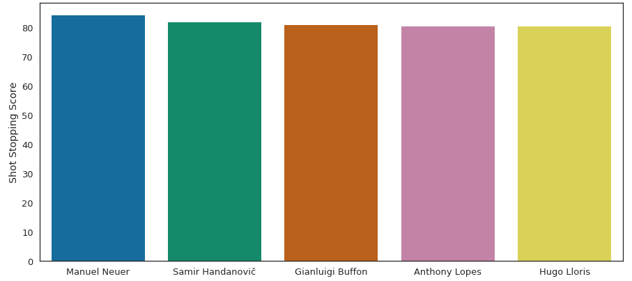
In order to get the best goalkeeper, I’ll be analyzing the data for the below mentioned parameters:
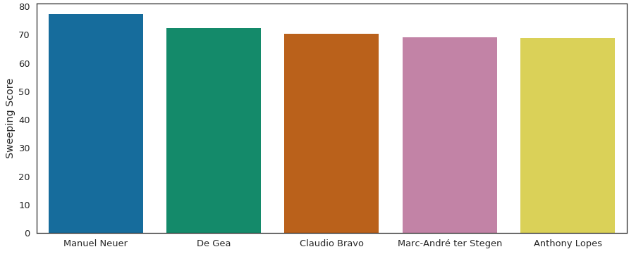
#weights
a = 0.5
b = 1
c= 2
d = 3

#GoalKeeping Characterstics
df['gk_Shot_Stopper'] = (b*df.Reactions + b*df.Composure + a*df.Speed + a*df.Strength + c*df.Jumping + b*df.GK_Positioning + c*df.GK_Diving + d*df.GK_Reflexes + b*df.GK_Handling)/(2*a + 4*b + 2*c + 1*d)
df['gk_Sweeper'] = (b*df.Reactions + b*df.Composure + b*df.Speed + a*df.Short_Pass + a*df.Long_Pass + b*df.Jumping + b*df.GK_Positioning + b*df.GK_Diving + d*df.GK_Reflexes + b*df.GK_Handling + d*df.GK_Kicking + c*df.Vision)/(2*a + 4*b + 3*c + 2*d)
Based on the above parameters, I’ll be predicting my best goalkeeper as per the dataset. Let us now plot these parameters:
plt.figure(figsize=(15,6))

# Generate sequential data and plot
sd = df.sort_values('gk_Shot_Stopper', ascending=False)[:5]
x1 = np.array(list(sd['Name']))
y1 = np.array(list(sd['gk_Shot_Stopper']))
sns.barplot(x1, y1, palette= "colorblind")
plt.ylabel("Shot Stopping Score")
plt.figure(figsize=(15,6))
sd = df.sort_values('gk_Sweeper', ascending=False)[:5]
x2 = np.array(list(sd['Name']))
y2 = np.array(list(sd['gk_Sweeper']))
sns.barplot(x2, y2, palette= "colorblind")
plt.ylabel("Sweeping Score")

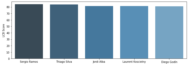
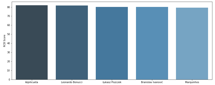
#Choosing Defenders
df['df_centre_backs'] = ( d*df.Reactions + c*df.Interceptions + d*df.Sliding_Tackle + d*df.Standing_Tackle + b*df.Vision+ b*df.Composure + b*df.Crossing +a*df.Short_Pass + b*df.Long_Pass+ c*df.Acceleration + b*df.Speed
+ d*df.Stamina + d*df.Jumping + d*df.Heading + b*df.Long_Shots + d*df.Marking + c*df.Aggression)/(6*b + 3*c + 7*d)
df['df_wb_Wing_Backs'] = (b*df.Ball_Control + a*df.Dribbling + a*df.Marking + d*df.Sliding_Tackle + d*df.Standing_Tackle + a*df.Attacking_Position + c*df.Vision + c*df.Crossing + b*df.Short_Pass + c*df.Long_Pass + d*df.Acceleration +d*df.Speed + c*df.Stamina + a*df.Finishing)/(4*a + 2*b + 4*c + 4*d)
plt.figure(figsize=(15,6))
sd = df[(df['Club_Position'] == 'LCB')].sort_values('df_centre_backs', ascending=False)[:5]
x2 = np.array(list(sd['Name']))
y2 = np.array(list(sd['df_centre_backs']))
sns.barplot(x2, y2, palette=sns.color_palette("Blues_d"))
plt.ylabel("LCB Score")
plt.figure(figsize=(15,6))

sd = df[(df['Club_Position'] == 'RCB')].sort_values('df_centre_backs', ascending=False)[:5]
x2 = np.array(list(sd['Name']))
y2 = np.array(list(sd['df_centre_backs']))
sns.barplot(x2, y2, palette=sns.color_palette("Blues_d"))
plt.ylabel("RCB Score")
plt.figure(figsize=(15,6))

sd = df[(df['Club_Position'] == 'LWB') | (df['Club_Position'] == 'LB')].sort_values('df_wb_Wing_Backs', ascending=False)[:5]
x4 = np.array(list(sd['Name']))
y4 = np.array(list(sd['df_wb_Wing_Backs']))
sns.barplot(x4, y4, palette=sns.color_palette("Blues_d"))
plt.ylabel("Left Back Score")
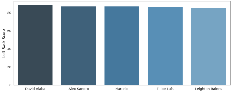
Since David Alaba’s team does not qualify in the world cup 2018, I’ll be picking Alex Sandro as the best LWB/LB defender.
plt.figure(figsize=(15,6))
sd = df[(df['Club_Position'] == 'RWB') | (df['Club_Position'] == 'RB')].sort_values('df_wb_Wing_Backs', ascending=False)[:5]
x5 = np.array(list(sd['Name']))
y5 = np.array(list(sd['df_wb_Wing_Backs']))
sns.barplot(x5, y5, palette=sns.color_palette("Blues_d"))
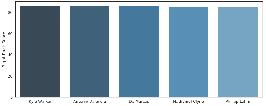
plt.ylabel("Right Back Score")

Moving ahead with the World’s Best Playing XI, it’s time we choose some midfielders.
#Midfielding Indices
df['mf_playmaker'] = (d*df.Ball_Control + d*df.Dribbling + a*df.Marking + d*df.Reactions + d*df.Vision + c*df.Attacking_Position + c*df.Crossing + d*df.Short_Pass + c*df.Long_Pass + c*df.Curve + b*df.Long_Shots + c*df.Freekick_Accuracy)/(1*a + 1*b + 4*c + 4*d)
df['mf_beast'] = (d*df.Agility + c*df.Balance + b*df.Jumping + c*df.Strength + d*df.Stamina + a*df.Speed + c*df.Acceleration + d*df.Short_Pass + c*df.Aggression + d*df.Reactions + b*df.Marking + b*df.Standing_Tackle + b*df.Sliding_Tackle + b*df.Interceptions)/(1*a + 5*b + 4*c + 4*d)
df['mf_controller'] = (b*df.Weak_foot + d*df.Ball_Control + a*df.Dribbling + a*df.Marking + a*df.Reactions + c*df.Vision + c*df.Composure + d*df.Short_Pass + d*df.Long_Pass)/(2*c + 3*d + 4*a)
Let us plot each one of them.
plt.figure(figsize=(15,6))
ss = df[(df['Club_Position'] == 'CAM') | (df['Club_Position'] == 'LAM') | (df['Club_Position'] == 'RAM')].sort_values('mf_playmaker', ascending=False)[:5]
x3 = np.array(list(ss['Name']))
y3 = np.array(list(ss['mf_playmaker']))
sns.barplot(x3, y3, palette=sns.diverging_palette(145, 280, s=85, l=25, n=5))
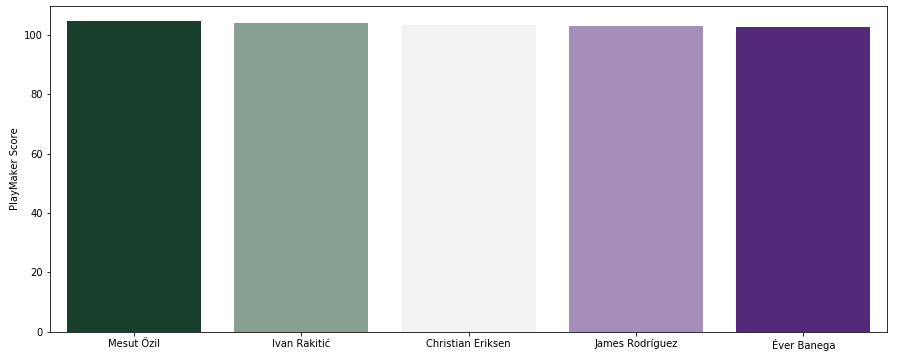
plt.ylabel("PlayMaker Score")
plt.figure(figsize=(15,6))
ss = df[(df['Club_Position'] == 'RCM') | (df['Club_Position'] == 'RM')].sort_values('mf_beast', ascending=False)[:5]
x2 = np.array(list(ss['Name']))
y2 = np.array(list(ss['mf_beast']))
sns.barplot(x2, y2, palette=sns.diverging_palette(145, 280, s=85, l=25, n=5))
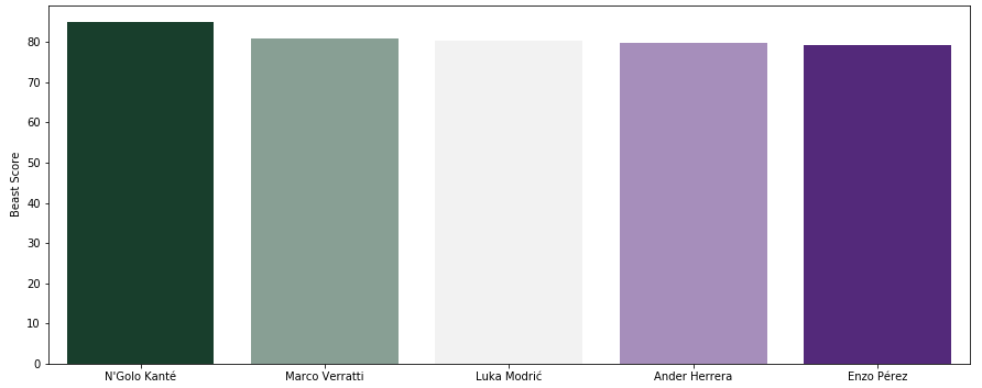
plt.ylabel("Beast Score")
plt.figure(figsize=(15,6))

# Generate some sequential data
ss = df[(df['Club_Position'] == 'LCM') | (df['Club_Position'] == 'LM')].sort_values('mf_controller', ascending=False)[:5]
x1 = np.array(list(ss['Name']))
y1 = np.array(list(ss['mf_controller']))
sns.barplot(x1, y1, palette=sns.diverging_palette(145, 280, s=85, l=25, n=5))
plt.ylabel("Controller Score")
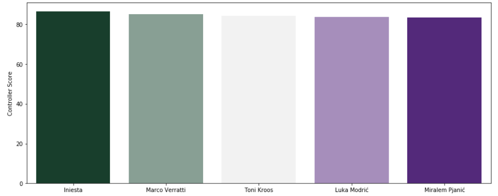
As per the above analysis, I’ll pick Iniesta as the best controller/ Left Central Midfielder.
Having said that, below is the list of the best mid-fielders for this World Cup 2018:

Moving ahead with the World’s Best Playing XI, it’s time we choose attackers.
#Attackers
df['att_left_wing'] = (c*df.Weak_foot + c*df.Ball_Control + c*df.Dribbling + c*df.Speed + d*df.Acceleration + b*df.Vision + c*df.Crossing + b*df.Short_Pass + b*df.Long_Pass + b*df.Aggression + b*df.Agility + a*df.Curve + c*df.Long_Shots + b*df.Freekick_Accuracy + d*df.Finishing)/(a + 6*b + 6*c + 2*d)
df['att_right_wing'] = (c*df.Weak_foot + c*df.Ball_Control + c*df.Dribbling + c*df.Speed + d*df.Acceleration + b*df.Vision + c*df.Crossing + b*df.Short_Pass + b*df.Long_Pass + b*df.Aggression + b*df.Agility + a*df.Curve + c*df.Long_Shots + b*df.Freekick_Accuracy + d*df.Finishing)/(a + 6*b + 6*c + 2*d)
df['att_striker'] = (b*df.Weak_foot + b*df.Ball_Control + a*df.Vision + b*df.Aggression + b*df.Agility + a*df.Curve + a*df.Long_Shots + d*df.Balance + d*df.Finishing + d*df.Heading + c*df.Jumping + c*df.Dribbling)/(3*a + 4*b + 2*c + 3*d)
Let us plot all of them and find the best attackers in the world for our best XI.
plt.figure(figsize=(15,6))

ss = df[(df['Club_Position'] == 'LW') | (df['Club_Position'] == 'LM') | (df['Club_Position'] == 'LS')].sort_values('att_left_wing', ascending=False)[:5]
x1 = np.array(list(ss['Name']))
y1 = np.array(list(ss['att_left_wing']))
sns.barplot(x1, y1, palette=sns.diverging_palette(255, 133, l=60, n=5, center="dark"))
plt.ylabel("Left Wing")
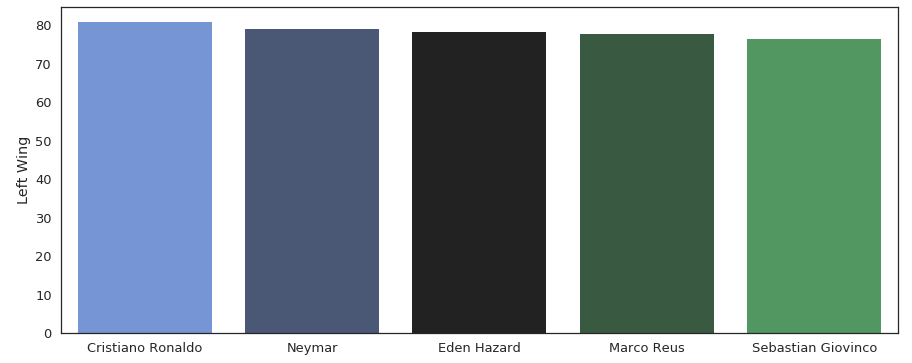
It’s quite evident from the above plot that Ronaldo is the best Left Wing Attacker for World Cup 2018.
Next, let us plot the right wing attacker.
plt.figure(figsize=(15,6))

ss = df[(df['Club_Position'] == 'RW') | (df['Club_Position'] == 'RM') | (df['Club_Position'] == 'RS')].sort_values('att_right_wing', ascending=False)[:5]
x2 = np.array(list(ss['Name']))
y2 = np.array(list(ss['att_right_wing']))
sns.barplot(x2, y2, palette=sns.diverging_palette(255, 133, l=60, n=5, center="dark"))
plt.ylabel("Right Wing")
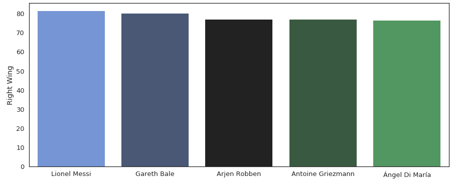
As per the above analysis, I’ll pick Lionel Messi as the right wing attacker for World Cup 2018.
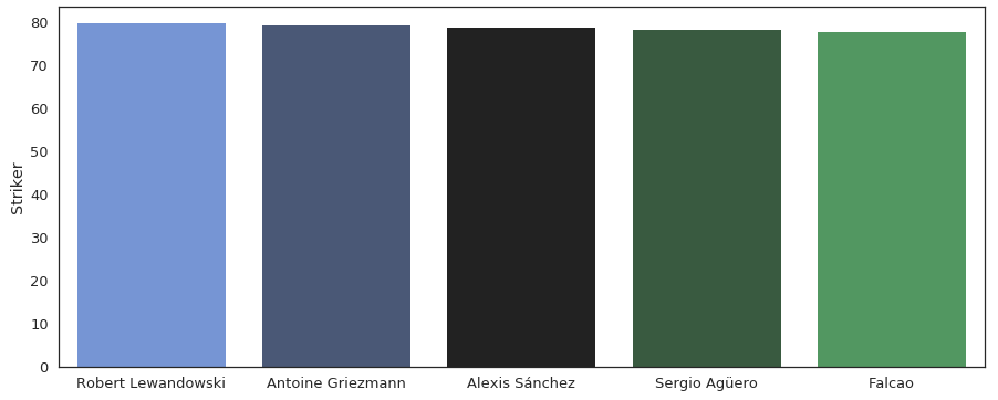
Moving ahead with the World’s Best Playing XI, it’s time we choose our striker.
plt.figure(figsize=(15,6))
ss = df[(df['Club_Position'] == 'ST') | (df['Club_Position'] == 'LS') | (df['Club_Position'] == 'RS') | (df['Club_Position'] == 'CF')].sort_values('att_striker', ascending=False)[:5]
x3 = np.array(list(ss['Name']))
y3 = np.array(list(ss['att_striker']))
sns.barplot(x3, y3, palette=sns.diverging_palette(255, 133, l=60, n=5, center="dark"))
plt.ylabel("Striker")


 Thank you for registering Join Edureka Meetup community for 100+ Free Webinars each month JOIN MEETUP GROUP
You have done a great job and I have learnt a lot.
Which algorithm is used for this prediction?