

Advanced Power BI Certification Course with G ...
- 13k Enrolled Learners
- Weekend
- Live Class
(4230)


 Copy Link!
Data is the most consistent raw material that was, is, and will be required in every era and the most popular tool that is used by almost everyone in the world to manage data is undoubtedly Microsoft Excel. Excel is used by almost every organization and with so much popularity and importance, it is certain that every individual must have knowledge of Excel. In case you don’t have your hands on it yet, don’t worry because this Excel tutorial will guide you through all that you need to know.
Here is a glimpse of all the topics that are discussed over here:
Microsoft Excel is a spreadsheet (computer application that allows storage of data in a tabular form) developed by Microsoft. It can be used on Windows, macOS, IOS, and Android platforms. Some of its features include:
Follow the steps given below to launch Excel:
Once this is done, you will see the following screen:
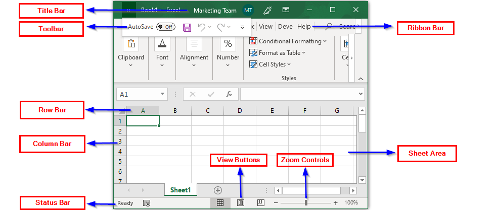
It displays the title of the sheet and appears right in the middle at the top of the Excel window.
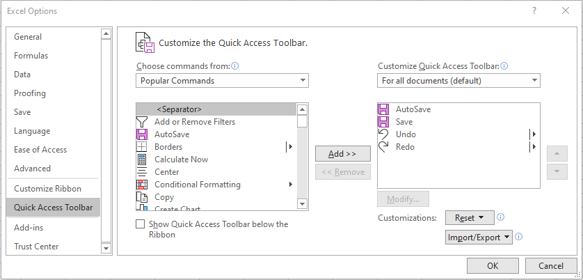
This toolbar consists of all commonly used Excel commands. In case you want to add some command that you use frequently to this toolbar, you can do it easily by customizing the quick access toolbar. To do that, right-click on it and select the option “Customize Quick Access Toolbar”. You will see the following window from where you can choose the appropriate commands that you would like to add.
The ribbon tab consists of the File, Home, Insert, Page Layout, View, etc tabs. The default tab that is selected by Excel is the Home tab. Just like the Quick Access Toolbar, you can also customize the Ribbon tab.
In order to customize the Ribbon tab, right-click anywhere on it and select the option “Customize the Ribbon”. You will see the following dialog box:
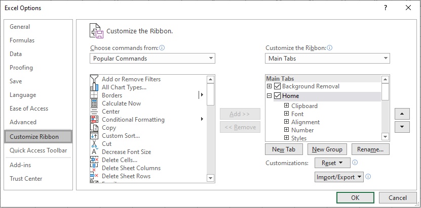
From here, you can select any tab that you want to add to the Ribbon bar according to your preference.
The Ribbon tab options are tailored into three components i.e Tabs, Groups and Commands. Tabs basically appear right on the top consisting of Home, Insert, file, etc. Groups consist of all related commands such as the font commands, insert commands, etc. Commands appear individually.
It allows you to zoom-in and zoom-out the sheet as and when required. To do this, you will just need to drag the slider towards the left side or the right side to zoom-in and zoom-out respectively.
Consists of three options namely, the Normal Layout View, Page Layout View, and the Page Break View. Normal Layout View displays the sheet in a normal view. Page Layout View allows you to see the page just like it would appear when you take a print out of it. The Page Break View basically shows where the page is going to break when you print it.
This is the area wherein the data will be inserted. The flashing vertical bar or the insertion point indicates the position of data insertion.
The Row bar shows the row numbers. It starts at 1 and the upper limit is 1,048,576 rows.
The Column bar shows the columns in the A-Z order. It starts at A and goes on till Z following which, it goes on as AA, AB, etc. The upper limit for columns is 16,384.
It is used to display the current status of the cell that is active in the sheet. There are four states namely Ready, Edit, Enter, and Point.
Ready, as the name suggests, is used to indicate that the worksheet can accept the user’s input.
Edit status indicates that the cell is in the editing-mode. In order to edit data of a cell, you can simply double click on that cell and enter the desired data.
Enter mode is enabled when the user starts to enter the data in the cell that is selected for editing.
Point mode is enabled when a formula is being entered into a cell with reference to the data present in some other cell.
The Backstage view is the central managing place for all your Excel sheets. From here, you can create, save, open print or share your worksheets. To go to the Backstage, simply click on File and you will see a column with a number of options which are described in the following table:
Option | Description |
New | Used to open a new Excel sheet |
Info | Gives information about the current worksheet |
Open | In order to open some sheets created earlier, you can use Open |
Close | Closes the open sheet |
Recent | Displays all the recently opened Excel sheets |
Share | Allows you to share the worksheet |
Save | To save the current sheet as it is, choose Save |
Save As | When you have to rename and select a particular file location for your sheet, you can use Save As |
USed to print the sheet | |
Export | Allows you to create a PDF or XPS document for your sheet |
Account | Contains all the account holders details |
Options | Shows all Excel options |
Refers to your Excel file itself. When you open the Excel app, click on the Blank workbook option to create a new Workbook.
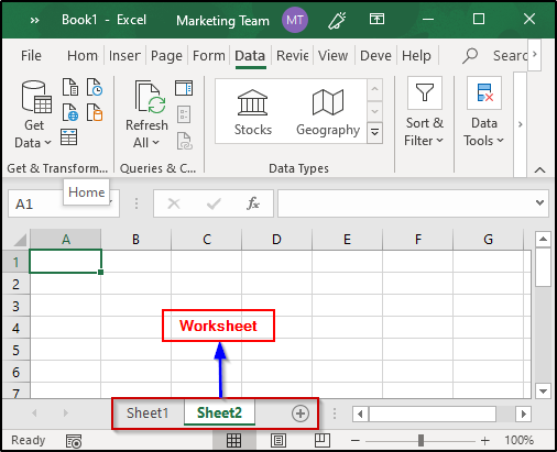
Refers to a collection of cells wherein you manage your data. Each Excel workbook can have multiple worksheets. These sheets will be displayed towards the bottom of the window, with their respective names as shown in the image below.
As mentioned earlier, the data is entered into the Sheet Area and the flashing vertical bar represents the cell and the place where your data will be entered in that cell. If you wish to choose some particular cell, just left-click on that cell and then double-click on it to enable the Enter mode. You can also Move around using the keyboard’s arrow keys.
To save your worksheet, click on the File tab and then select the Save As option. Select the appropriate folder where you would like to save the sheet and save it with an appropriate name. The default format in which an Excel file will be saved is .xlsx format.
In case you make changes to an existing file, you can just press Ctrl+S or open the File tab and select Save option. Excel also provides the Floppy Icon in the Quick Access toolbar to help you save your worksheet easily.
To create a new Worksheet, click on the + icon present next to the current Worksheet as shown in the image below:

You can also right-click on the Worksheet and select the Insert option to create a new Worksheet. Excel also provides a shortcut to create a new Worksheet i.e using Shift+F11.
In case you have a Worksheet and you want to create another copy of it, you can do as follows:

A dialog box will appear where you have the options to move the sheet at the required position and at the end of that dialog box, you will see an option as ‘Create a copy’. By checking that box, you will be able to create a copy of an existing sheet.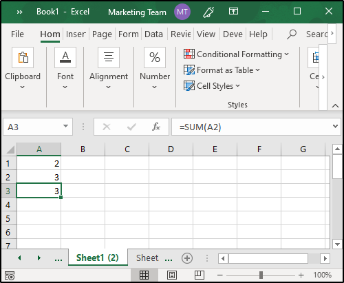
You can also left-click on the sheet and drag it to the required position in order to move the sheet. To rename the file, double-click on the desired file and rename it.
In order to hide a worksheet, right-click on the name of that sheet and select the Hide option. Conversely, if you want to undo this, right-click on any of the sheet names and select Unhide option. You will see a dialog box that contains all the hidden sheets, select the sheet that you want to unhide and click on OK.
To delete a sheet, right-click on the sheet name and select the Delete option. In case the sheet is empty, it will be deleted or else you will see a dialog box warning you that you might lose the data stored in that particular sheet.
To close a Workbook, click on the File tab, and then select the Close option. You will see a dialog box asking you to optionally save the changes that have made to the Workbook in the desired directory.
To open a previously created Workbook, click on the File tab and select the Open option. You will see all the worksheets that have created previously when you select Open. left-click on the file that you intend to open.
Excel has a very special feature called the context help feature that provides appropriate information about the Excel commands in order to educate the user about its working as shown in the image below:
The total number of cells present in an excel sheet is 16,384 x 1,048,576. The type of data i.e entered can be in any form such as textual, numerical or formulae.
In order to enter the data, simply select the cell wherein you intend to insert the data and type the same. In case of formulas, you will need to enter them either directly in the cell or in the formula bar that is provided on top as shown in the image below:
there are two ways to select Excel data. The first and simplest way is to make use of the mouse. Just click on the required and cell and double click on it. Also, in case you want to select a complete section of data entries, hold left-click and drag it down till that cell which you intend to select. You can also hold the Ctrl button and left-click on random cells to select them.
The method is to use the Go To dialog box. To activate this box, you can either click on the Home tab and select the Find and Select option or simply click Ctrl+G. You will see a dialog box appearing that will have an option “Special”. Click on that option and you will see another dialog box as shown in the image below:
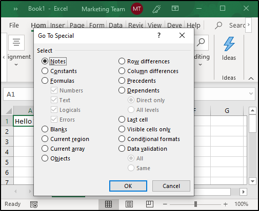
From here, check the appropriate region that you want to select and click on OK. Once this is done, you will see that the entire region of your choice has been selected.
In order to delete some data, you can use the following techniques:
Excel also allows you to move your data easily to the desired location. You can do this in just two simple steps:
If you want to Copy and Paste data in Excel, you can do it in the following ways:
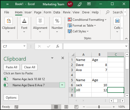
Excel also provides a Clipboard that will hold all the data that you have copied. In case you want to paste any of that data, simply select it from the Clipboard and choose the paste option as shown below:
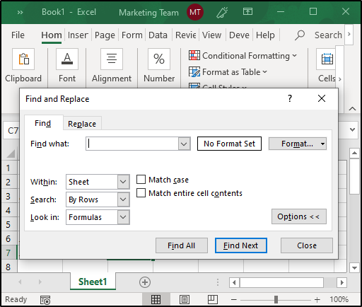
To Find and Replace data, you can either select the Find & Replace option from the Home tab or simply press Ctrl+F You will a dialog box that will have all the related options to find and replace the require data.
In case you need to enter a symbol that is not present on the keyboard, you can make use of the Special Symbols provided in Excel where you will find Equations and Symbols. In order to select these Symbols, click on the Insert tab and select Symbols option. You will have two options namely Equation and Symbols as shown below:

If you select Equation, you will find a number equations such as the Area of a circle, the Binomial Theorem, Expansion of a Sum, etc. If you select the Symbol, you will see the following dialog box:
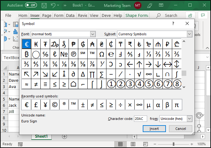
You can select any Symbol of your choice and click on the Insert option.
In order to give a clear description of the data, it is important to add comments. Excel allows you to add, modify and format comments.
Adding a Comment or a Note:
You can add comments and notes as follows:
The comment dialog box will hold the user name of the system which can be replaced by the appropriate comments.
To edit a note, right-click on the cell that has the note and chose the Edit Note option and update it accordingly. In case you don’t need the note anymore, right-click on the cell containing it and choose the Delete Note option.
In case of a Comment, just select the cell containing the comment and it will open the comment dialog box from where you can edit or delete the comments. You can also reply to comments specified by other users working on that sheet.
Cells of an Excel sheet can be formatted for the various types of data that they can hold. There are a number of ways to format the cells.
Setting the cell type:
The cells of an Excel sheet can be set to a particular type such as General, Number, Currency, Accounting, etc. To do this, right-click on the cell to which you intend to specify some particular type of data and then select Format cells option. You will see a dialog box as shown in the image below that will have a number of options to select from.
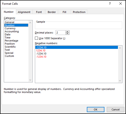
Type | Description |
General | No specific format |
Number | General display of numbers |
Currency | The cell will be displayed as a currency |
Accounting | It is similar to currency type but used for accounts |
Date | Allows various types of date formats |
Time | Allows various types of time formats |
Percentage | Cell displayed as a percentage |
Fraction | The cell is displayed as a fraction |
Scientific | Displays the cell in exponential form |
Text | For Normal text data |
Special | You can enter the special type of formats such as a phone number, ZIP, etc |
Custom | Allows Custom formats |
You can modify the font on an Excel sheet as follows:
In case you want to modify the look of the data, you can do so using the various options such as bold, italic, underline, etc that are present the same dialog box as shown in the image above or from the Home tab. You can select the effects options which are Strikethrough, Superscript, and Subscript.
Cells of an Excel sheet can be rotated to any degree. To do this, click on the Orientation group tab present within Home and select the type of orientation you desire.
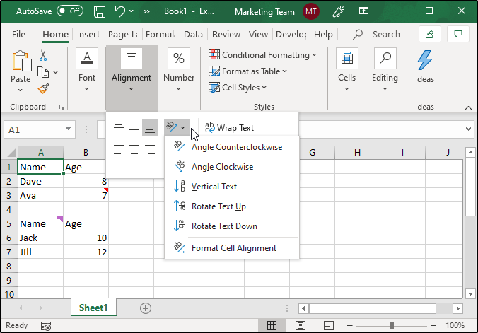
This can also be done from the Format cell dialog box by selecting the Alignment option. You also have options for aligning your data in various ways such as Top, Center, Justify, etc and you can change the direction as well using Context, Left-to-Right, and Right-to-Left options.
The cells of an MS Excel sheet can be merged and unmerged as and when required. Keep the following points in mind when you merge cells of an Excel sheet:
To merge cells, simply select all the cells you wish to merge and then select the Merge and Control option present in the Home tab or check the Merge cells option present in the Alignment window.
In case the cell holds a lot of data that starts to highlight other cells, you can use the Shrink to fit/ Wrap text options in order to reduce the size or align the text vertically.
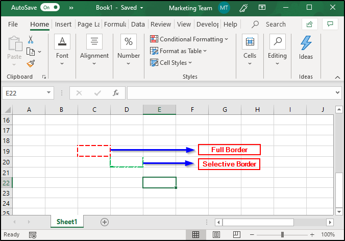
In case you want to add borders and shades to a cell in your worksheet, select that cell and right-click over it and select the Format cells option.
To add borders, open the Border window from the Format cells window and then choose the type of border that you would like to add to that cell. You can also vary the thickness, color, etc.
In case you want to add some shade to a cell, select that cell and then open the Fill pane from the Format cells window then choose the appropriate color of your choice.
Excel sheets provide a number of options for taking appropriate print outs. Using these options, you can selectively print your sheet in various ways. To open the sheet options pane, select Page Layout Group from the Home tab and open the Page Setup. Here, you will see a number of sheet options that are listed in the table below:
Option | Description |
Print Area | Sets the print area |
Print Titles | Allows you to set the row and column titles to appear at the top and towards the left respectively |
Gridlines | Gridlines will be added to the printout |
Black and White | Print out is black and white or monochrome |
Draft Quality | Prints the sheet using your printers Draft quality |
Row and Column Headings | Allows you to print row and column headings |
Down, then over | Prints the down pages first followed by the right pages |
Over, then down | Prints the right pages first and then the down page |
The unprinted regions along the top-down and left-right sides are referred to as margins. All MS Excel pages have a border and if you have selected some border for one page, then that border will be applied to all the pages i.e you can’t have different margins for each page. You can add margins as follows:
Page Orientations refer to the format in which the sheet is printed i.e Portrait and Landscape. The Portrait orientation is default and prints the page taller than wide. On the other hand, the Landscape orientation prints the sheet wider than tall.
To select a particular type of page orientation, select the drop-down list from the Page Setup group or maximize the Page Setup window and choose the appropriate orientation. You can also change the page orientation while printing the MS Excel sheet just like how you did with Margins.
Headers and Footers are used to provide some information at the top and at the bottom of the page. A new workbook does not have a Header or a Footer. In order to add it, you can open the Page Setup window and then open the Header/ Footer pane. Here, you will have a number of options to customize the Headers and Footers. If you want to preview the Header and Footers that you have added, click on the Print Preview option and you will be able to see the changes that you have made.
MS Excel allows you to precisely control what you want to print and what you want to omit. Using Page Breaks, you will be able to control the print of the page such as restrain from printing the first row of a table at the end of a page or printing the header of a new page at the end of the previous page. Using page breaks will allow you to print the sheet in the order of your preference. You can have both Horizontal as well as Vertical page breaks. To include this, select the row or column where you intend to include a page break and then from the Page Setup group, select the option Insert Page Break.
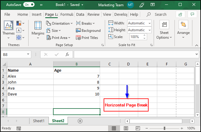
Horizontal Page Break:
To introduce a Horizontal Page Break, select the row where you want the page to break from. Take a look at the image below where I have introduced a Horizontal Page Break in order to print the row A4 on the next page.
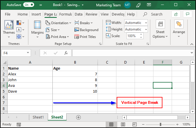
Vertical Page Break:
To introduce a Vertical Page Break, select the column where you want the page to break from. Take a look at the image below where I have introduced a Vertical Page Break.
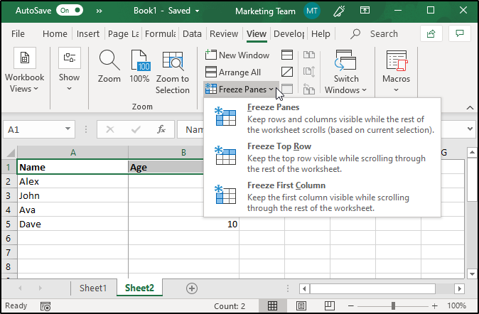
MS Excel provides an option of freezing panes which will enable you to see the row and column headings even if you keep scrolling down the page. In order to Freeze Panes, you will have to:
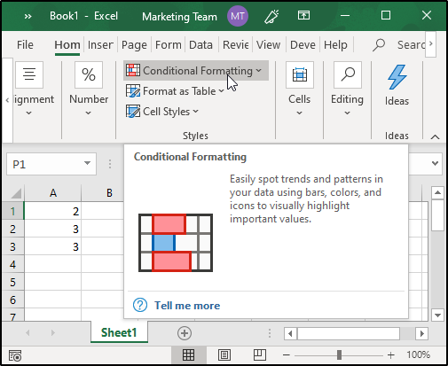
Conditional Formatting allows you to selectively format a section to hold values within some specified range. Values outside these ranges will be formatted automatically. This feature has a number of options which are listed in the table below:
Option | Description |
Highlight Cells Rules | Opens another list that defines the selected cells contain values, text or dates that are greater than, equal to, less than some particular value |
Top/ Bottom Rules | Highlights the top/ bottom values, percents, as well as the upper and lower averages |
Data Bars | Opens up a palette with differently colored data bars |
Color Scales | Contains a color palette with two and three colored scales |
Icon Sets | Contains different sets of icons |
New Rule | Opens up a New Formatting rule dialog box for custom conditional formatting |
Clear Rules | Allows you to remove the conditional formatting rules |
Manage Rules | Conditional Formatting Rules Manager dialog box opens up from where you can add, delete or format rules according to your preference |
Formulas are one of the most important features of an Excel sheet. A formula is basically an expression that can be entered into the cells and the output of that particular expression is displayed in that cell as the output. The formulas of an MS Excel sheet can be:
MS Excel allows you to enter formulas by a number of means such as:
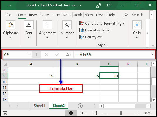
For creating a formula, you will have to exclusively enter a formula in the formula bar of the sheet. The formula should always start with a “=” sign. You can manually build your formula by specifying cell addresses or just by pointing to the cell in the worksheet.
You can copy Excel sheet formulas in case you have to calculate some common results. Excel automatically handles the task of copying formulas where ever similar ones are needed.
Relative Cell Addresses:
Like I have mentioned before, Excel automatically manages cell references of the original formula in order to match the position where it is copied. This task is accomplished through a system known as Relative Cell Addresses. Here, the copied formula will have modified row and column addresses that will suit its new position.
In order to copy a formula, select a cell that holds the original formula and drag it until the cell that you want to calculate the formula for. For example, in the previous example, I have calculated the sum of A9 and B9. Now, to calculate the sum of A10 and B10, all I have to do is, select C9 and drag it down to C10 as shown in the image below:
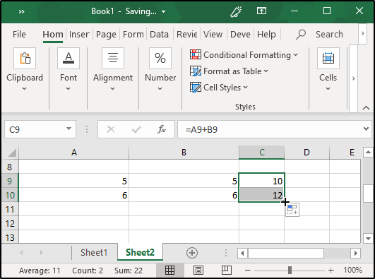
As you can see, the formula is copied without me having to exclusively specify the cell addresses.
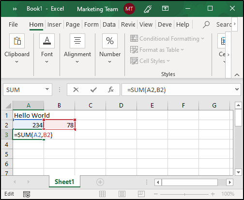
Most of the Excel formulas are with reference to the cell or a range of cell addresses that enable you to work with the data dynamically. For example, if I change the value of any of the cells in the previous example, the result will be updated automatically.
This addressing can be of three types namely relative, absolute or mixed.
Relative Cell Address:
When you copy a formula, the row and column references change accordingly. This is because the cell references are actually the offsets from the current column or row.
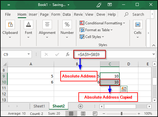
Absolute Cell Reference:
The row and column address do not get modified when copied as the reference points to the original cell itself. Absolute references are created using $ signs in the address preceding the column letter and the row number. For example, $A$9 is an absolute address.
Mixed Cell Reference:
Here, either the cell or column is absolute and the other is relative. Take a look at the image below: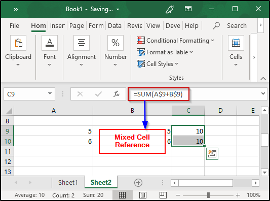
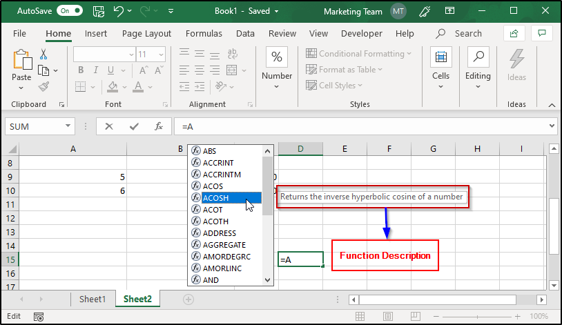
Functions available in MS Excel actually handle many of the formulas that you create. These functions actually define complex calculations that are difficult to manually define using just operators. Excel provides many functions and if you want some particular function, all you have to do is type in the first letter of that function in the formula bar and Excel will display a drop-down list holding all the functions that start with that letter. Not just this, hen you hover the mouse over these function names, Excel brilliantly gives a description about it. Take a look at the image below:
Excel provides a huge number of built-in functions that you can use in any of your formulas. to look out for all the functions, click on fx and then you will see a window opening that will have all Excel’s built-in functions. From here you can select any function based on the category to which it belongs.
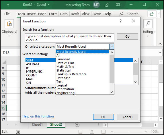
Some of the most important built-in Excel Functions include If STATEMENTS, SUMIF, COUNTIF, VLOOKUP, HLOOKUP, CONCATENATE, MAX, MIN, etc.
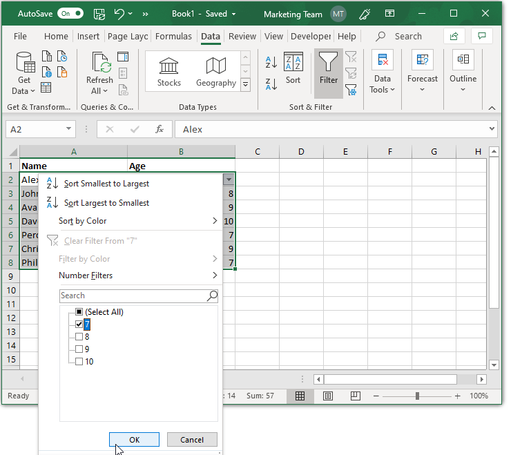
Filtering the data basically means to pull out data from those rows and columns that meet some specific conditions. In this case, the other rows or columns get hidden. For example, if you have a list of student Names with their Ages, and if you want to filter out only those students that are of 7 years, all you have to do is, select a specific range of cells and from the Data tab, click on the Filter command. Once this is done, you will be able to see a drop-down list as shown in the image below:
Advanced Excel tutorial includes all the topics that will help you learn to manage real-time data using excel sheets. It includes using complex Excel functions, creating charts, filtering data, pivot charts and pivot tables, data charts and tables, etc.
This brings us to the end of this article on Excel Tutorial. I hope you are clear with all that has been shared with you. Make sure you practice as much as possible and revert your experience. Supercharge your Excel skills with our complete guide to formulas and functions, and Excel Interview questions for your next interview with confidence!
Also, If you’re looking to improve your abilities and learn more about Data Visualization to become certified as a Business Intelligence Professional. Go through our Tableau Training Course now to get all the information you should learn about this powerful software.
Also Read:
How do you use an advanced filter to filter by date in Excel?
Count Specific Characters in Google Sheets How to count specific characters in google sheets?


 Thank you for registering Join Edureka Meetup community for 100+ Free Webinars each month JOIN MEETUP GROUP