


Data Science and Machine Learning Internship ...
- 22k Enrolled Learners
- Weekend/Weekday
- Live Class
(8500)
A Decision Tree has many analogies in real life and turns out, it has influenced a wide area of Machine Learning, covering both Classification and Regression. In decision analysis, a decision tree can be used to visually and explicitly represent decisions and decision making.
So the outline of what I’ll be covering in this blog is as follows.
A decision tree is a map of the possible outcomes of a series of related choices. It allows an individual or organization to weigh possible actions against one another based on their costs, probabilities, and benefits.
As the name goes, it uses a tree-like model of decisions. They can be used either to drive informal discussion or to map out an algorithm that predicts the best choice mathematically.
A decision tree typically starts with a single node, which branches into possible outcomes. Each of those outcomes leads to additional nodes, which branch off into other possibilities. This gives it a tree-like shape.
There are three different types of nodes: chance nodes, decision nodes, and end nodes. A chance node, represented by a circle, shows the probabilities of certain results. A decision node, represented by a square, shows a decision to be made, and an end node shows the final outcome of a decision path.
Let us consider a scenario where a new planet is discovered by a group of astronomers. Now the question is whether it could be ‘the next earth?’ The answer to this question will revolutionize the way people live. Well, literally!
There is n number of deciding factors which need to be thoroughly researched to take an intelligent decision. These factors can be whether water is present on the planet, what is the temperature, whether the surface is prone to continuous storms, flora and fauna survives the climate or not, etc.
Let us create a decision tree to find out whether we have discovered a new habitat.
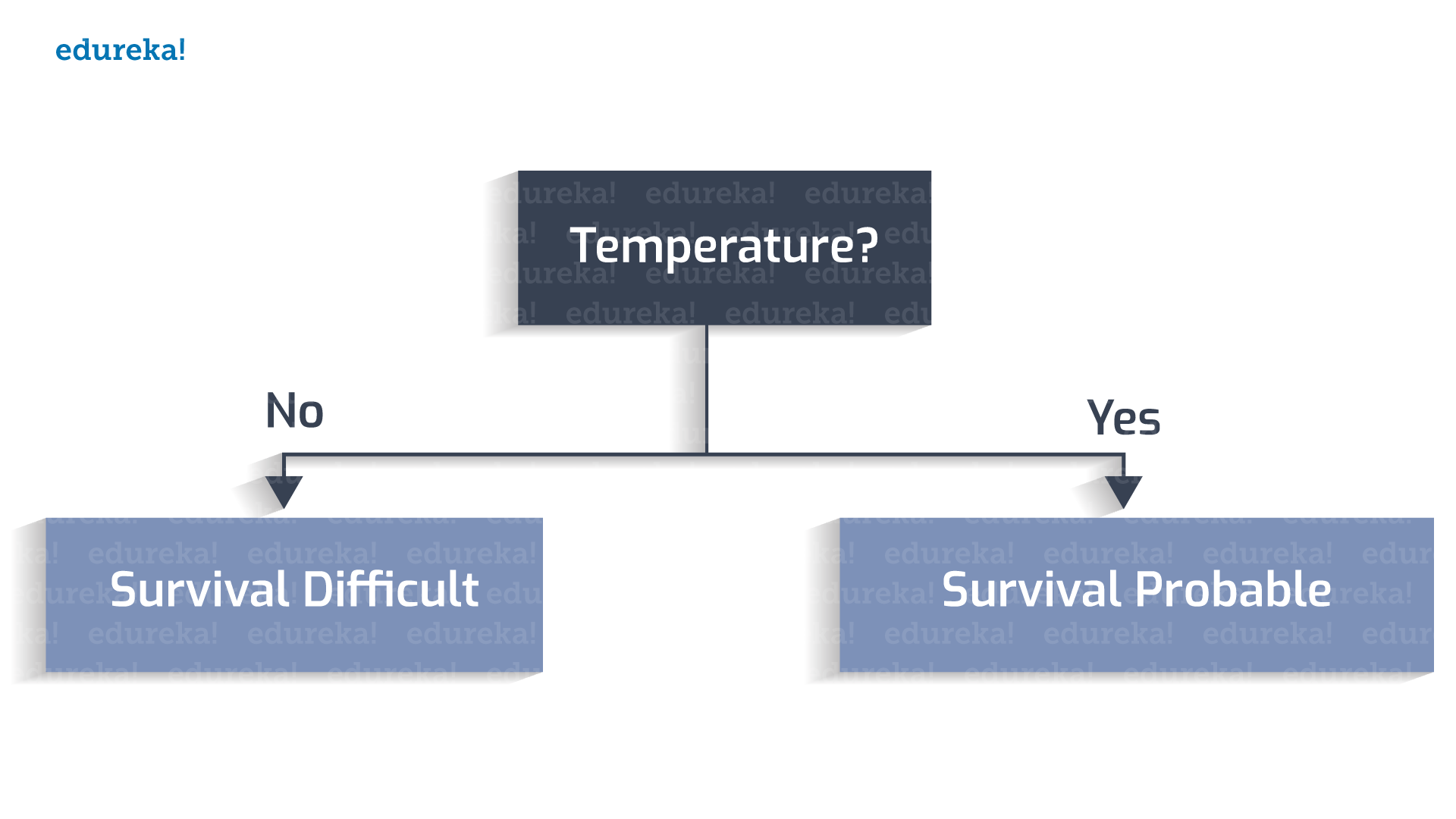
The habitable temperature falls into the range 0 to 100 Celsius.
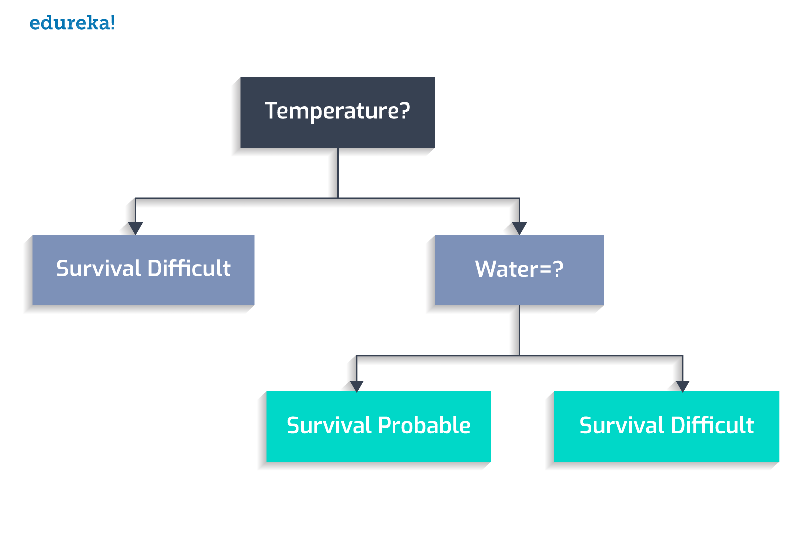
 Whether water is present or not?
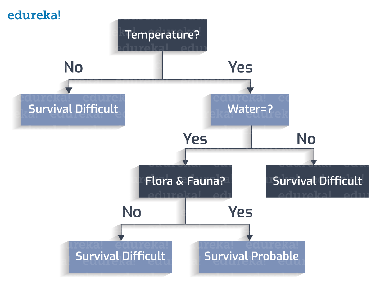
 Whether flora and fauna flourishes?
 The planet has a stormy surface?
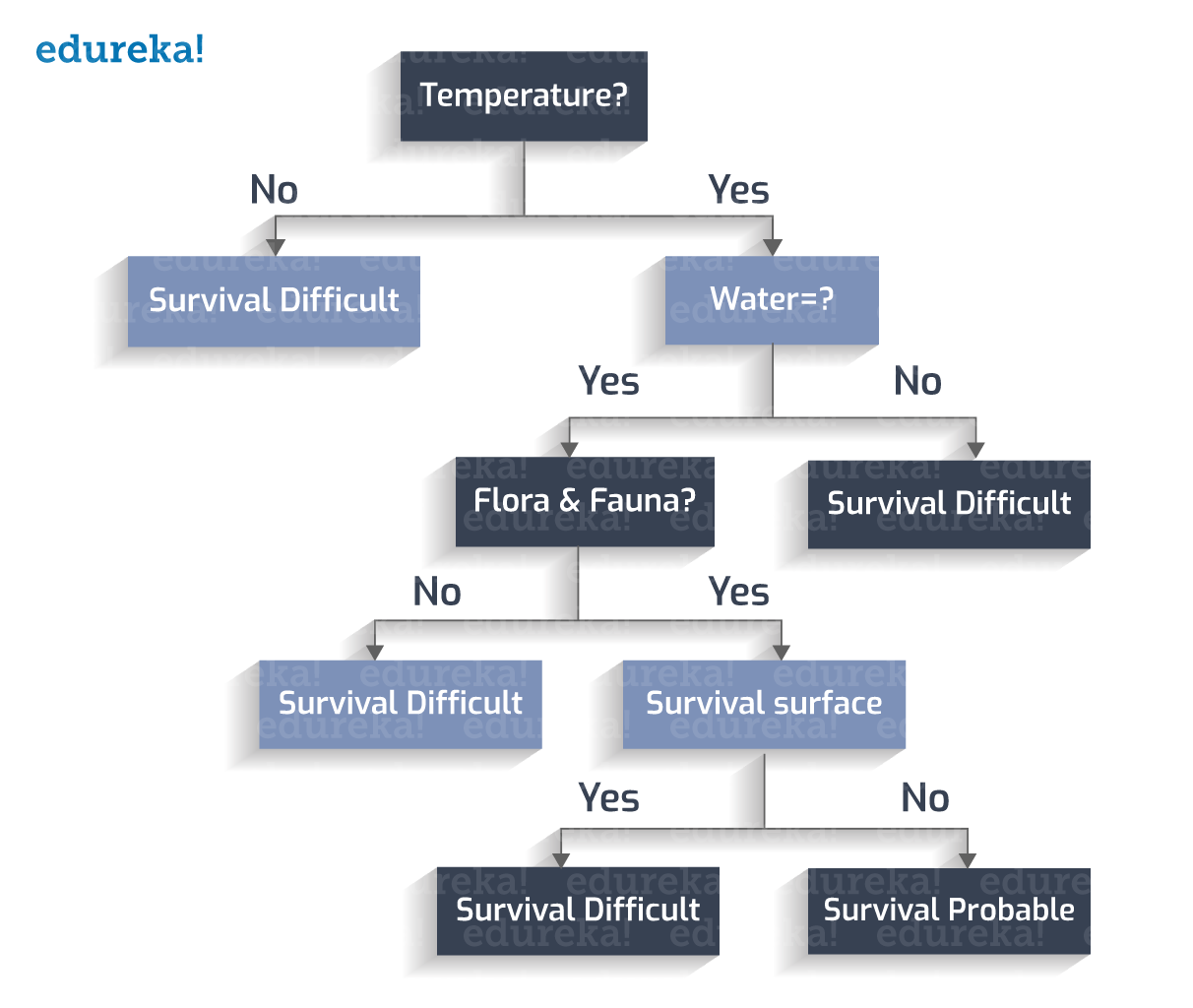 Thus, we a have a decision tree with us.
Classification rules are the cases in which all the scenarios are taken into consideration and a class variable is assigned to each.
Each leaf node is assigned a class-variable. A class-variable is the final output which leads to our decision.
Let us derive the classification rules from the Decision Tree created:
1. If Temperature is not between 273 to 373K, -> Survival Difficult
2. If Temperature is between 273 to 373K, and water is not present, -> Survival Difficult
3. If Temperature is between 273 to 373K, water is present, and flora and fauna is not present -> Survival Difficult
4. If Temperature is between 273 to 373K, water is present, flora and fauna is present, and a stormy surface is not present -> Survival Probable
5. If Temperature is between 273 to 373K, water is present, flora and fauna is present, and a stormy surface is present -> Survival Difficult
A decision tree has the following constituents :
As the decision tree is now constructed, starting from the root-node we check the test condition and assign the control to one of the outgoing edges, and so the condition is again tested and a node is assigned. The decision tree is said to be complete when all the test conditions lead to a leaf node. The leaf node contains the class-labels, which vote in favor or against the decision.
Now, you might think why did we start with the ‘temperature’ attribute at the root? If you choose any other attribute, the decision tree constructed will be different.
Correct. For a particular set of attributes, there can be numerous different trees created. We need to choose the optimal tree which is done by following an algorithmic approach. We will now see ‘the greedy approach’ to create a perfect decision tree.
“Greedy Approach is based on the concept of Heuristic Problem Solving by making an optimal local choice at each node. By making these local optimal choices, we reach the approximate optimal solution globally.”
The algorithm can be summarized as :
1. At each stage (node), pick out the best feature as the test condition.
2. Now split the node into the possible outcomes (internal nodes).
3. Repeat the above steps till all the test conditions have been exhausted into leaf nodes.
When you start to implement the algorithm, the first question is: ‘How to pick the starting test condition?’
The answer to this question lies in the values of ‘Entropy’ and ‘Information Gain’. Let us see what are they and how do they impact our decision tree creation.
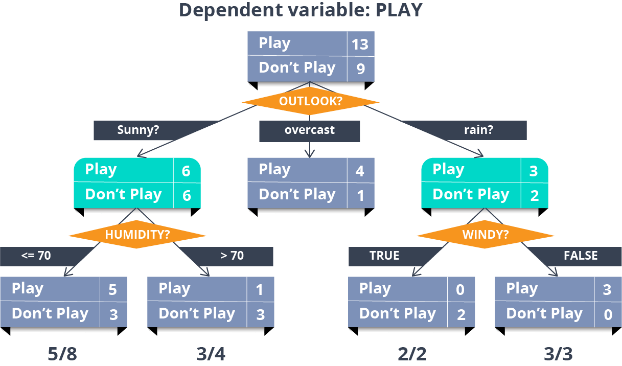
Entropy: Entropy in Decision Tree stands for homogeneity. If the data is completely homogenous, the entropy is 0, else if the data is divided (50-50%) entropy is 1.
Information Gain: Information Gain is the decrease/increase in Entropy value when the node is split.
An attribute should have the highest information gain to be selected for splitting. Based on the computed values of Entropy and Information Gain, we choose the best attribute at any particular step.
Let us consider the following data:
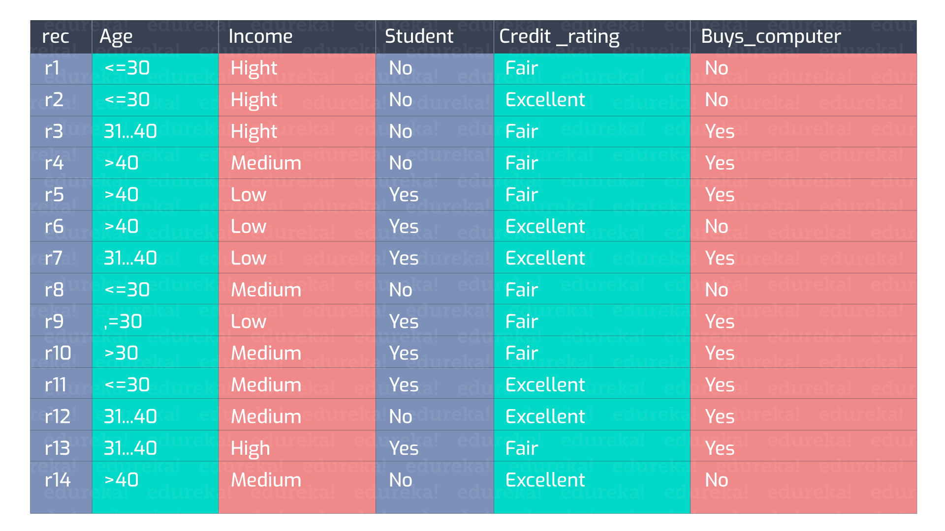 There can be n number of decision trees that can be formulated from these set of attributes.
Here we take up the attribute ‘Student’ as the initial test condition.
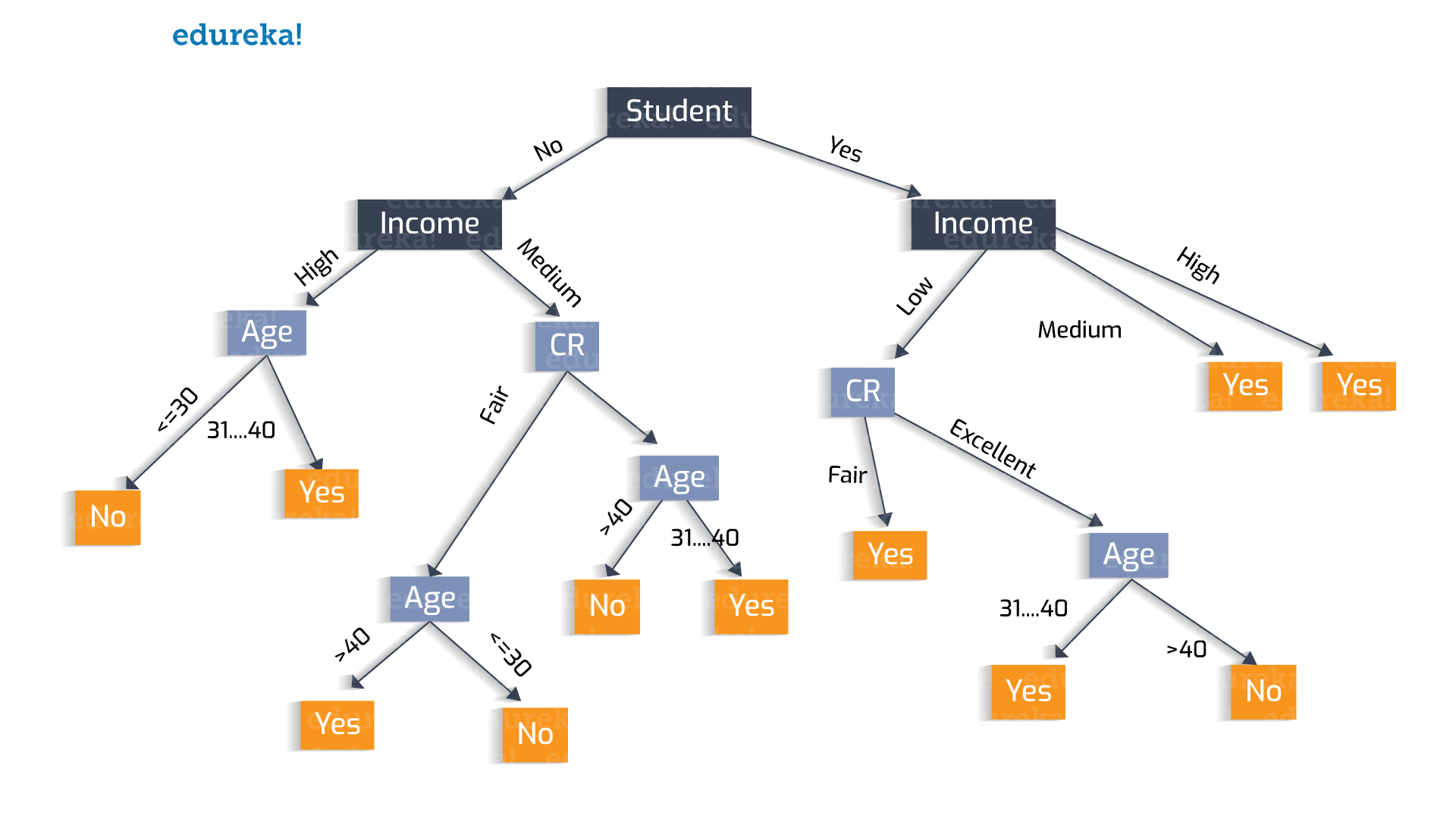
Similarly, why to choose ‘Student’? We can choose ‘Income’ as the test condition.
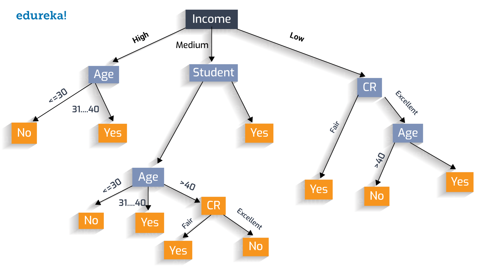
Let us follow the ‘Greedy Approach’ and construct the optimal decision tree.

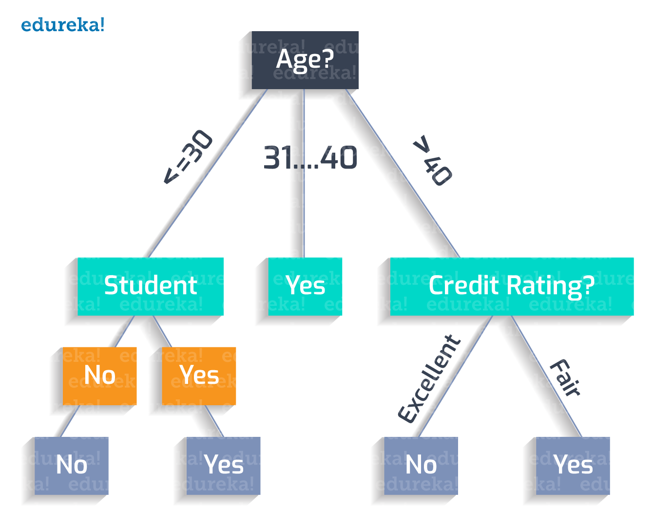 The classification rules for this tree can be jotted down as:
Age(<30) ^ student(no) = NO
If a person’s age is less than 30 and he is a student, he will buy the product.
Age(<30) ^ student(yes) = YES
If a person’s age is between 31 and 40, he is most likely to buy.
Age(31…40) = YES
If a person’s age is greater than 40 and has an excellent credit rating, he will not buy.
Age(>40) ^ credit_rating(excellent) = NO
If a person’s age is greater than 40, with a fair credit rating, he will probably buy.
Age(>40) ^ credit_rating(fair) = Yes
Thus, we achieve the perfect Decision Tree!!
Now that you have gone through our Decision Tree blog, you can check out Edureka’s Data Science Certification Training. Got a question for us? Please mention it in the comments section and we will get back to you.


 REGISTER FOR FREE WEBINAR
  Thank you for registering Join Edureka Meetup community for 100+ Free Webinars each month JOIN MEETUP GROUP


Very Good :)
Thanks Pratik!!