A Complete Guide On Decision Tree Algorithm

With the increase in the implementation of Machine Learning algorithms for solving industry level problems, the demand for more complex and iterative algorithms has become a need. The Decision Tree Algorithm is one such algorithm that is used to solve both Regression and Classification problems.

In this blog on Decision Tree Algorithm, you will learn the working of Decision Tree and how it can be implemented to solve real-world problems. The following topics will be covered in this blog:

1. Why Decision Tree?
2. What Is A Decision Tree?
3. How Does The Decision Tree Algorithm Work?
4. Building A Decision Tree
5. Practical Implementation Of Decision Tree Algorithm Using R

To get in-depth knowledge on Data Science, you can enroll for live Data Science Certification Training by Edureka with 24/7 support and lifetime access.

Before I get started with why use Decision Tree, here’s a list of Machine Learning blogs that you should go through to understand the basics:

• Machine Learning Algorithms
• Introduction To Classification Algorithms
• Random Forest Classifier

We’re all aware that there are n number of Machine Learning algorithms that can be used for analysis, so why should you choose Decision Tree? In the below section I’ve listed a few reasons.

Why Decision Tree Algorithm?

Decision Tree is considered to be one of the most useful Machine Learning algorithms since it can be used to solve a variety of problems. Here are a few reasons why you should use Decision Tree:

1. It is considered to be the most understandable Machine Learning algorithm and it can be easily interpreted.
2. It can be used for classification and regression problems.
3. Unlike most Machine Learning algorithms, it works effectively with non-linear data.
4. Constructing a Decision Tree is a very quick process since it uses only one feature per node to split the data.

What Is A Decision Tree Algorithm?

To get a better understanding of a Decision Tree, let’s look at an example:

Let’s say that you hosted a huge party and you want to know how many of your guests were non-vegetarians. To solve this problem, let’s create a simple Decision Tree.

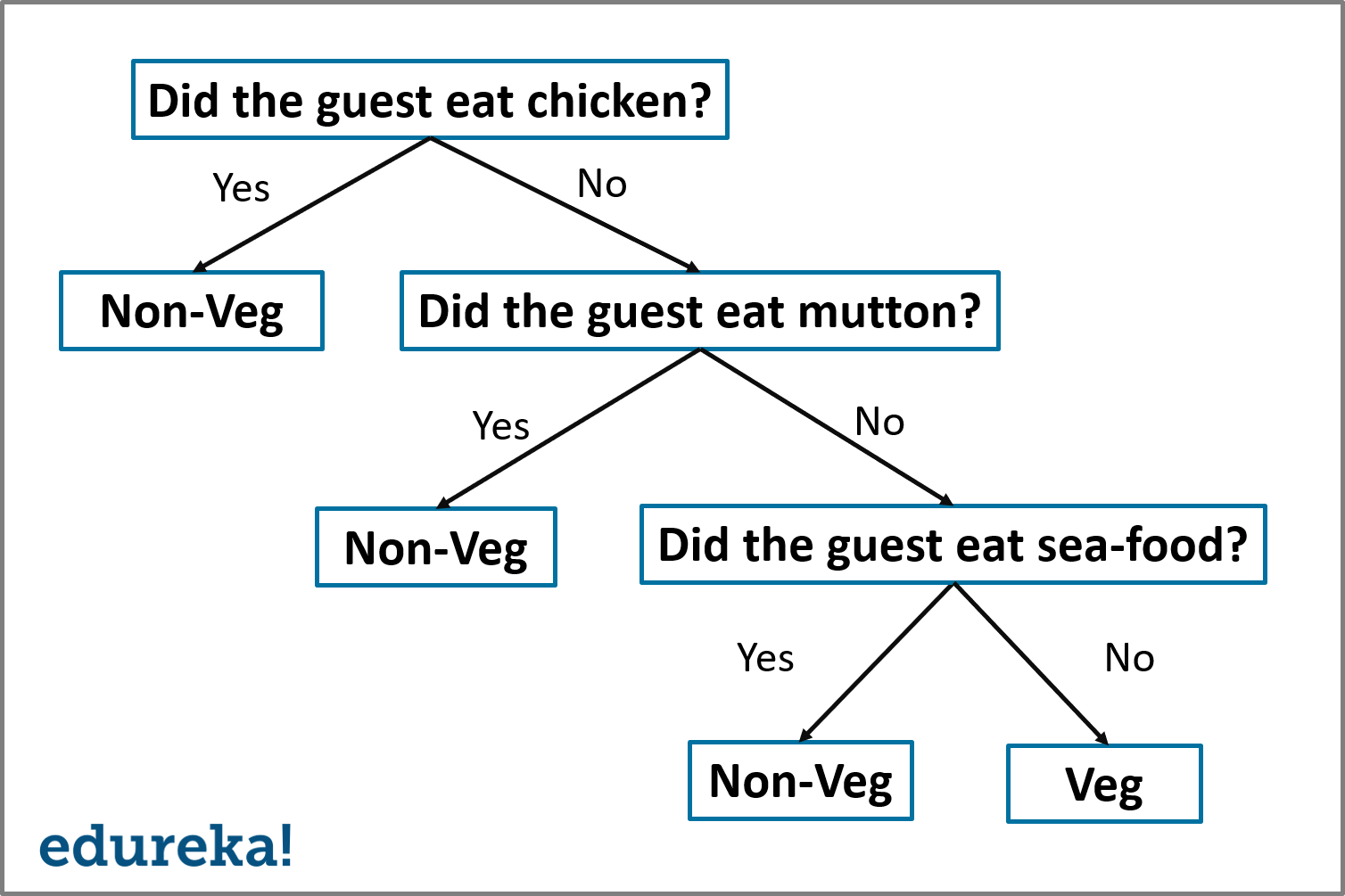
Decision Tree Example – Decision Tree Algorithm – Edureka

In the above illustration, I’ve created a Decision tree that classifies a guest as either vegetarian or non-vegetarian. Each node represents a predictor variable that will help to conclude whether or not a guest is a non-vegetarian. As you traverse down the tree, you must make decisions at each node, until you reach a dead end.

Now that you know the logic of a Decision Tree, let’s define a set of terms related to a Decision Tree.

Structure Of A Decision Tree

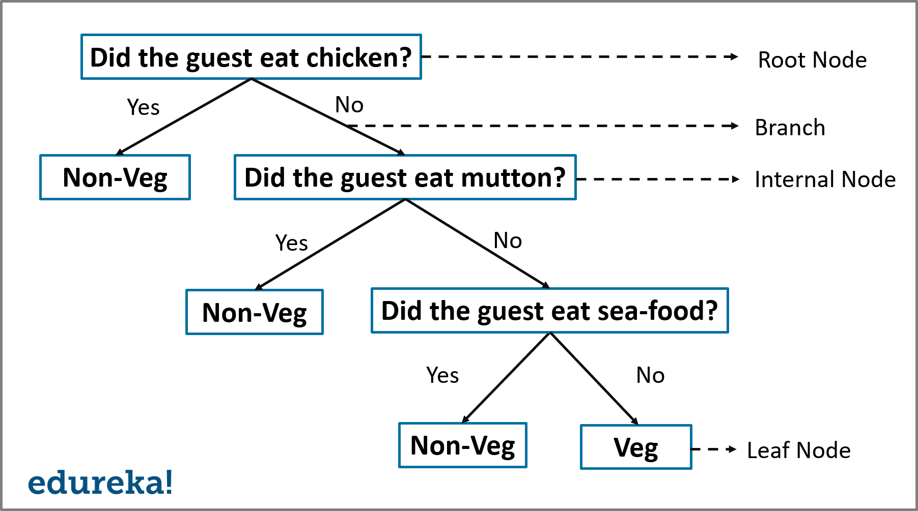
Decision Tree Structure – Decision Tree Algorithm – Edureka

A Decision Tree has the following structure:

• Root Node: The root node is the starting point of a tree. At this point, the first split is performed.
• Internal Nodes: Each internal node represents a decision point (predictor variable) that eventually leads to the prediction of the outcome.
• Leaf/ Terminal Nodes: Leaf nodes represent the final class of the outcome and therefore they’re also called terminating nodes.
• Branches: Branches are connections between nodes, they’re represented as arrows. Each branch represents a response such as yes or no.

So that is the basic structure of a Decision Tree. Now let’s try to understand the workflow of a Decision Tree.

How Does The Decision Tree Algorithm Work?

The Decision Tree Algorithm follows the below steps:

Step 1: Select the feature (predictor variable) that best classifies the data set into the desired classes and assign that feature to the root node.
Step 2: Traverse down from the root node, whilst making relevant decisions at each internal node such that each internal node best classifies the data.
Step 3: Route back to step 1 and repeat until you assign a class to the input data.

The above-mentioned steps represent the general workflow of a Decision Tree used for classification purposes.

Now let’s try to understand how a Decision Tree is created.

Build A Decision Tree Using ID3 Algorithm

There are many ways to build a Decision Tree, in this blog we’ll be focusing on how the ID3 algorithm is used to create a Decision Tree.

What Is The ID3 Algorithm?

ID3 or the Iterative Dichotomiser 3 algorithm is one of the most effective algorithms used to build a Decision Tree. It uses the concept of Entropy and Information Gain to generate a Decision Tree for a given set of data.

ID3 Algorithm:

The ID3 algorithm follows the below workflow in order to build a Decision Tree:

1. Select Best Attribute (A)
2. Assign A as a decision variable for the root node.
3. For each value of A, build a descendant of the node.
4. Assign classification labels to the leaf node.
5. If data is correctly classified: Stop.
6. Else: Iterate over the tree.

The first step in this algorithm states that we must select the best attribute. What does that mean?

The best attribute (predictor variable) is the one that, separates the data set into different classes, most effectively or it is the feature that best splits the data set. 

Now the next question in your head must be, “How do I decide which variable/ feature best splits the data?”

Two measures are used to decide the best attribute:

1. Information Gain
2. Entropy

What Is Entropy?

What Is Information Gain?

Information Gain is important because it used to choose the variable that best splits the data at each node of a Decision Tree. The variable with the highest IG is used to split the data at the root node.

Equation For Information Gain (IG):

To better understand how Information Gain and Entropy are used to create a Decision Tree, let’s look at an example. The below data set represents the speed of a car based on certain parameters.

Speed Data Set – Decision Tree Algorithm – Edureka

Your problem statement is to study this data set and create a Decision Tree that classifies the speed of a car (response variable) as either slow or fast, depending on the following predictor variables:

• Road type
• Obstruction
• Speed limit

We’ll be building a Decision Tree using these variables in order to predict the speed of a car. Like I mentioned earlier we must first begin by deciding a variable that best splits the data set and assign that particular variable to the root node and repeat the same thing for the other nodes as well.

At this point, you might be wondering how do you know which variable best separates the data? The answer is, the variable with the highest Information Gain best divides the data into the desired output classes.

So, let’s begin by calculating the Entropy and Information Gain (IG) for each of the predictor variables, starting with ‘Road type’.

In our data set, there are four observations in the ‘Road type’ column that correspond to four labels in the ‘Speed of car’ column. We shall begin by calculating the entropy of the parent node (Speed of car).

Step one is to find out the fraction of the two classes present in the parent node. We know that there are a total of four values present in the parent node, out of which two samples belong to the ‘slow’ class and the other 2 belong to the ‘fast’ class, therefore:

• P(slow) -> fraction of ‘slow’ outcomes in the parent node
• P(fast) -> fraction of ‘fast’ outcomes in the parent node

The formula to calculate P(slow) is:

p(slow) = no. of ‘slow’ outcomes in the parent node / total number of outcomes

Similarly, the formula to calculate P(fast) is:

p(fast) = no. of ‘fast’ outcomes in the parent node / total number of outcomes

Therefore, the entropy of the parent node is:

Entropy(parent) = – {0.5 log2(0.5) + 0.5 log2(0.5)} = – {-0.5 + (-0.5)} = 1

Now that we know that the entropy of the parent node is 1, let’s see how to calculate the Information Gain for the ‘Road type’ variable. Remember that, if the Information gain of the ‘Road type’ variable is greater than the Information Gain of all the other predictor variables, only then the root node can be split by using the ‘Road type’ variable.

In order to calculate the Information Gain of ‘Road type’ variable, we first need to split the root node by the ‘Road type’ variable.

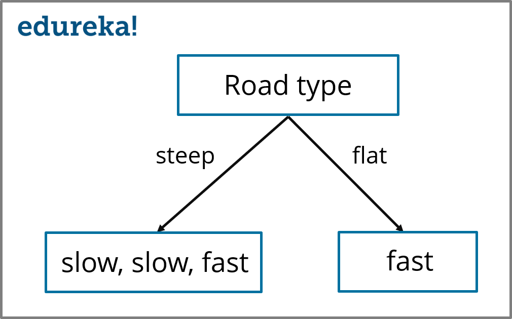Decision Tree (Road type) – Decision Tree Algorithm – Edureka

In the above illustration, we’ve split the parent node by using the ‘Road type’ variable, the child nodes denote the corresponding responses as shown in the data set. Now, we need to measure the entropy of the child nodes.

The entropy of the right-hand side child node (fast) is 0 because all of the outcomes in this node belongs to one class (fast). In a similar manner, we must find the Entropy of the left-hand side node (slow, slow, fast).

In this node there are two types of outcomes (fast and slow), therefore, we first need to calculate the fraction of slow and fast outcomes for this particular node.

P(slow) = 2/3 = 0.667
P(fast) = 1/3 = 0.334

Therefore, entropy is:

Entropy(left child node) = – {0.667 log2(0.667) + 0.334 log2(0.334)} = – {-0.38 + (-0.52)}
= 0.9

Our next step is to calculate the Entropy(children) with weighted average:

• Total number of outcomes in parent node: 4
• Total number of outcomes in left child node: 3
• Total number of outcomes in right child node: 1

Formula for Entropy(children) with weighted avg. :

By using the above formula you’ll find that the, Entropy(children) with weighted avg. is = 0.675

Our final step is to substitute the above weighted average in the IG formula in order to calculate the final IG of the ‘Road type’ variable:

Therefore,

Information gain(Road type) = 1 – 0.675 = 0.325

Information gain of Road type feature is 0.325.

Like I mentioned earlier, the Decision Tree Algorithm selects the variable with the highest Information Gain to split the Decision Tree. Therefore, by using the above method you need to calculate the Information Gain for all the predictor variables to check which variable has the highest IG.

So by using the above methodology, you must get the following values for each predictor variable:

1. Information gain(Road type) = 1 – 0.675 = 0.325
2. Information gain(Obstruction) = 1 – 1 = 0
3. Information gain(Speed limit) = 1 – 0 = 1

So, here we can see that the ‘Speed limit’ variable has the highest Information Gain. Therefore, the final Decision Tree for this dataset is built using the ‘Speed limit’ variable.

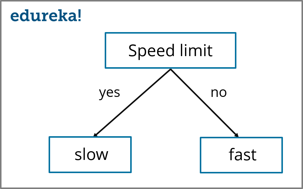
Decision Tree (Speed limit) – Decision Tree Algorithm – Edureka

Now that you know how a Decision Tree is created, let’s run a short demo that solves a real-world problem by implementing Decision Trees.

Implementation Of Decision Tree In R – Decision Tree Algorithm Example

Problem Statement: To study a Mushroom data set in order to predict whether a given mushroom is edible or poisonous to human beings.

Data Set Description: The given data set contains a total of 8124 observations of different kind of mushrooms and their properties such as odor, habitat, population, etc. A more in-depth structure of the data set is shown in the demo below. 

Logic: To build a Decision Tree model in order to classify mushroom samples as either poisonous or edible by studying their properties such as odor, root, habitat, etc.

Now that you know the objective of this demo, let’s get our brains working and start coding. For this demo, I’ll be using the R language in order to build the model.

If you wish to learn more about R programming, you can go through this video recorded by our R Programming Experts.

Now, let’s begin.

Step 1: Install and load libraries

#Installing libraries
install.packages('rpart')
install.packages('caret')
install.packages('rpart.plot')
install.packages('rattle')

#Loading libraries
library(rpart,quietly = TRUE)
library(caret,quietly = TRUE)
library(rpart.plot,quietly = TRUE)
library(rattle)

Step 2: Import the data set

#Reading the data set as a dataframe
mushrooms <- read.csv ("/Users/zulaikha/Desktop/decision_tree/mushrooms.csv")

Now, to display the structure of the data set, you can make use of the R function called str():

# structure of the data
> str(mushrooms)
'data.frame': 8124 obs. of 22 variables:
$ class : Factor w/ 2 levels "e","p": 2 1 1 2 1 1 1 1 2 1 ...
$ cap.shape : Factor w/ 6 levels "b","c","f","k",..: 6 6 1 6 6 6 1 1 6 1 ...
$ cap.surface : Factor w/ 4 levels "f","g","s","y": 3 3 3 4 3 4 3 4 4 3 ...
$ cap.color : Factor w/ 10 levels "b","c","e","g",..: 5 10 9 9 4 10 9 9 9 10 ...
$ bruises : Factor w/ 2 levels "f","t": 2 2 2 2 1 2 2 2 2 2 ...
$ odor : Factor w/ 9 levels "a","c","f","l",..: 7 1 4 7 6 1 1 4 7 1 ...
$ gill.attachment : Factor w/ 2 levels "a","f": 2 2 2 2 2 2 2 2 2 2 ...
$ gill.spacing : Factor w/ 2 levels "c","w": 1 1 1 1 2 1 1 1 1 1 ...
$ gill.size : Factor w/ 2 levels "b","n": 2 1 1 2 1 1 1 1 2 1 ...
$ gill.color : Factor w/ 12 levels "b","e","g","h",..: 5 5 6 6 5 6 3 6 8 3 ...
$ stalk.shape : Factor w/ 2 levels "e","t": 1 1 1 1 2 1 1 1 1 1 ...
$ stalk.root : Factor w/ 5 levels "?","b","c","e",..: 4 3 3 4 4 3 3 3 4 3 ...
$ stalk.surface.above.ring: Factor w/ 4 levels "f","k","s","y": 3 3 3 3 3 3 3 3 3 3 ...
$ stalk.surface.below.ring: Factor w/ 4 levels "f","k","s","y": 3 3 3 3 3 3 3 3 3 3 ...
$ stalk.color.above.ring : Factor w/ 9 levels "b","c","e","g",..: 8 8 8 8 8 8 8 8 8 8 ...
$ stalk.color.below.ring : Factor w/ 9 levels "b","c","e","g",..: 8 8 8 8 8 8 8 8 8 8 ...
$ veil.color : Factor w/ 4 levels "n","o","w","y": 3 3 3 3 3 3 3 3 3 3 ...
$ ring.number : Factor w/ 3 levels "n","o","t": 2 2 2 2 2 2 2 2 2 2 ...
$ ring.type : Factor w/ 5 levels "e","f","l","n",..: 5 5 5 5 1 5 5 5 5 5 ...
$ spore.print.color : Factor w/ 9 levels "b","h","k","n",..: 3 4 4 3 4 3 3 4 3 3 ...
$ population : Factor w/ 6 levels "a","c","n","s",..: 4 3 3 4 1 3 3 4 5 4 ...
$ habitat : Factor w/ 7 levels "d","g","l","m",..: 6 2 4 6 2 2 4 4 2 4 ...

The output shows a number of predictor variables that are used to predict the output class of a mushroom (poisonous or edible).

Step 3: Data Cleaning

At this stage, we must look for any null or missing values and unnecessary variables so that our prediction is as accurate as possible. In the below code snippet I have deleted the ‘veil.type’ variable since it has no effect on the outcome. Such inconsistencies and redundant data must be fixed in this step.

# number of rows with missing values
nrow(mushrooms) - sum(complete.cases(mushrooms))

# deleting redundant variable `veil.type`
mushrooms$veil.type <- NULL

Step 4: Data Exploration and Analysis

To get a good understanding of the 21 predictor variables, I’ve created a table for each predictor variable vs class type (response/ outcome variable) in order to understand whether that particular predictor variable is significant for detecting the output or not.

I’ve shown the table only for the ‘odor’ variable, you can go ahead and create a table for each of the variables by following the below code snippet:

# analyzing the odor variable
> table(mushrooms$class,mushrooms$odor)
a      c      f       l       m       n       p        s      y
e   400     0      0     400     0    3408    0       0      0
p   0      192   2160  0      36     120    256  576  576

In the above snippet, ‘e’ stands for edible class and ‘p’ stands for the poisonous class of mushrooms.

The above output shows that the mushrooms with odor values ‘c’, ‘f’, ‘m’, ‘p’, ‘s’ and ‘y’ are clearly poisonous. And the mushrooms having almond (a) odor (400) are edible. Such observations will help us to predict the output class more accurately.

Our next step in the data exploration stage is to predict which variable would be the best one for splitting the Decision Tree. For this reason, I’ve plotted a graph that represents the split for each of the 21 variables, the output is shown below:

number.perfect.splits <- apply(X=mushrooms[-1], MARGIN = 2, FUN = function(col){
t <- table(mushrooms$class,col)
sum(t == 0)
})

# Descending order of perfect splits
order <- order(number.perfect.splits,decreasing = TRUE)
number.perfect.splits <- number.perfect.splits[order]

# Plot graph
par(mar=c(10,2,2,2))
barplot(number.perfect.splits,
main="Number of perfect splits vs feature",
xlab="",ylab="Feature",las=2,col="wheat")

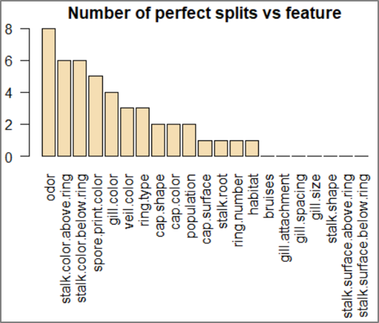
rpart.plot – Decision Tree Algorithm – Edureka

The output shows that the ‘odor’ variable plays a significant role in predicting the output class of the mushroom.

Step 5: Data Splicing

Data Splicing is the process of splitting the data into a training set and a testing set. The training set is used to build the Decision Tree model and the testing set is used to validate the efficiency of the model. The splitting is performed in the below code snippet:

#data splicing
set.seed(12345)
train <- sample(1:nrow(mushrooms),size = ceiling(0.80*nrow(mushrooms)),replace = FALSE)
# training set
mushrooms_train <- mushrooms[train,]
# test set
mushrooms_test <- mushrooms[-train,]

To make this demo more interesting and to minimize the number of poisonous mushrooms misclassified as edible we will assign a penalty 10x bigger, than the penalty for classifying an edible mushroom as poisonous because of obvious reasons. 

# penalty matrix
penalty.matrix <- matrix(c(0,1,10,0), byrow=TRUE, nrow=2)

Step 6: Building a model

In this stage, we’re going to build a Decision Tree by using the rpart  (Recursive Partitioning And Regression Trees) algorithm:

# building the classification tree with rpart
tree <- rpart(class~.,
data=mushrooms_train,
parms = list(loss = penalty.matrix),
method = "class")

Step 7: Visualising the tree

In this step, we’ll be using the rpart.plot library to plot our final Decision Tree:

# Visualize the decision tree with rpart.plot
rpart.plot(tree, nn=TRUE)

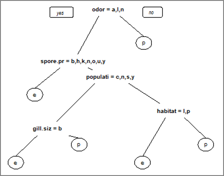
Decision Tree – Decision Tree Algorithm – Edureka

Step 8: Testing the model

Now in order to test our Decision Tree model, we’ll be applying the testing data set on our model like so:

#Testing the model
pred <- predict(object=tree,mushrooms_test[-1],type="class")

Step 9: Calculating accuracy

We’ll be using a confusion matrix to calculate the accuracy of the model. Here’s the code:

#Calculating accuracy
t <- table(mushrooms_test$class,pred) > confusionMatrix(t)
Confusion Matrix and Statistics

pred
e&nbsp; &nbsp; &nbsp; p
e&nbsp; 839&nbsp; &nbsp; 0
p&nbsp; 0&nbsp; &nbsp; &nbsp;785

Accuracy : 1
95% CI : (0.9977, 1)
No Information Rate : 0.5166
P-Value [Acc > NIR] : < 2.2e-16

Kappa : 1
Mcnemar's Test P-Value : NA

Sensitivity : 1.0000
Specificity : 1.0000
Pos Pred Value : 1.0000
Neg Pred Value : 1.0000
Prevalence : 0.5166
Detection Rate : 0.5166
Detection Prevalence : 0.5166
Balanced Accuracy : 1.0000

'Positive' Class : e

The output shows that all the samples in the test dataset have been correctly classified and we’ve attained an accuracy of 100% on the test data set with a 95% confidence interval (0.9977, 1). Thus we can correctly classify a mushroom as either poisonous or edible using this Decision Tree model.

Now that you know how the Decision Tree Algorithm works, I’m sure you’re curious to learn more about the various Machine learning algorithms. Here’s a list of blogs that cover the different types of Machine Learning algorithms in depth:

• Linear Regression
• Logistic Regression
• Support Vector Machine
• Random Forest
• K-Means

So, with this, we come to the end of this blog. I hope you all found this blog informative. If you have any thoughts to share, please comment them below. Stay tuned for more blogs like these!

If you are looking for online structured training in Data Science, edureka! has a specially curated Data Science course which helps you gain expertise in Statistics, Data Wrangling, Exploratory Data Analysis, Machine Learning Algorithms like K-Means Clustering, Decision Trees, Random Forest, Naive Bayes. You’ll learn the concepts of Time Series, Text Mining and an introduction to Deep Learning as well. New batches for this course are starting soon!!