
Data Science with Python Certification Course
- 131k Enrolled Learners
- Weekend
- Live Class
(49300)


 Copy Link!
_1648290501.jpg)
With the exponential outburst of AI, companies are eagerly looking to hire skilled Data Scientists to grow their business. Apart from getting a Data Science Certification, it is always good to have a couple of Data Science Projects on your resume. Having theoretical knowledge is never enough. So, in this blog, you’ll learn how to practically use Data Science methodologies to solve real-world problems.
Given the right data, Data Science can be used to solve problems ranging from fraud detection and smart farming to predicting climate change and heart diseases. With that being said, data isn’t enough to solve a problem, you need an approach or a method that will give you the most accurate results. This brings us to the question:
A problem statement in Data Science can be solved by following the below steps:
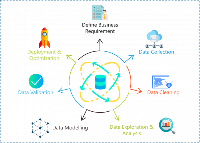
Data Science Project Life Cycle – Data Science Projects – Edureka
Let’s look at each of these steps in detail:
Step 1: Define Problem Statement
Before you even begin a Data Science project, you must define the problem you’re trying to solve. At this stage, you should be clear with the objectives of your project.
Step 2: Data Collection
Like the name suggests at this stage you must acquire all the data needed to solve the problem. Collecting data is not very easy because most of the time you won’t find data sitting in a database, waiting for you. Instead, you’ll have to go out, do some research and collect the data or scrape it from the internet.
Step 3: Data Cleaning
If you ask a Data Scientist what their least favorite process in Data Science is, they’re most probably going to tell you that it is Data Cleaning. Data cleaning is the process of removing redundant, missing, duplicate and unnecessary data. This stage is considered to be one of the most time-consuming stages in Data Science. However, in order to prevent wrongful predictions, it is important to get rid of any inconsistencies in the data.
Step 4: Data Analysis and Exploration
Once you’re done cleaning the data, it is time to get the inner Sherlock Holmes out. At this stage in a Data Science life-cycle, you must detect patterns and trends in the data. This is where you retrieve useful insights and study the behavior of the data. At the end of this stage, you must start to form hypotheses about your data and the problem you are tackling.
Step 5: Data Modelling
This stage is all about building a model that best solves your problem. A model can be a Machine Learning Algorithm that is trained and tested using the data. This stage always begins with a process called Data Splicing, where you split your entire data set into two proportions. One for training the model (training data set) and the other for testing the efficiency of the model (testing data set).
This is followed by building the model by using the training data set and finally evaluating the model by using the test data set.
Step 6: Optimization and Deployment:
This is the last stage of the Data Science life-cycle. At this stage, you must try to improve the efficiency of the data model, so that it can make more accurate predictions. The end goal is to deploy the model into production or production-like environment for final user acceptance. The users must validate the performance of the models and if there are any issues with the model then they must be fixed in this stage.
Now that you know how a problem can be solved using Data Science, let’s get to the fun part. In the following section, I will be providing you with five high-level Projects on Data Science that can get you hired in the top IT firms.
Before we start coding, here’s a short disclaimer:
I’m going to be using the R language to run the entire Data Science workflow because R is a statistical language and it has over 8000 packages that make our lives easier.
If you wish to learn more about R Programming, you can check out this video by our R Programming experts.
This Edureka R Tutorial will help you in understanding the fundamentals of R tool and help you build a strong foundation in R.
Problem Statement: To build a model that will predict if the income of any individual in the US is greater than or less than USD 50,000 based on the data available about that individual.
Data Set Description: This Census Income dataset was collected by Barry Becker in 1994 and given to the public site http://archive.ics.uci.edu/ml/datasets/Census+Income. This data set will help you understand how the income of a person varies depending on various factors such as the education background, occupation, marital status, geography, age, number of working hours/week, etc.
Here’s a list of the independent or predictor variables used to predict whether an individual earns more than USD 50,000 or not:
The dependent variable is the “income-level” that represents the level of income. This is a categorical variable and thus it can only take two values:
Now that we’ve defined our objective and collected the data, it is time to start with the analysis.
Step 1: Import the data
Lucky for us, we found a data set online, so all we have to do is import the data set into our R environment, like so:
#Downloading train and test data
trainFile = "adult.data"; testFile = "adult.test"

if (!file.exists (trainFile))
download.file (url = "http://archive.ics.uci.edu/ml/machine-learning-databases/adult/adult.data",
destfile = trainFile)

if (!file.exists (testFile))
download.file (url = "http://archive.ics.uci.edu/ml/machine-learning-databases/adult/adult.test",
destfile = testFile)
In the above code snippet, we’ve downloaded both, the training data set and the testing data set.
If you take a look at the training data, you’ll notice that the predictor variables are not labelled. Therefore, in the below code snippet, I’ve assigned variable names to each predictor variable and to make the data more readable, I’ve gotten rid of unnecessary white spaces.
#Assigning column names
colNames = c ("age", "workclass", "fnlwgt", "education",
"educationnum", "maritalstatus", "occupation",
"relationship", "race", "sex", "capitalgain",
"capitalloss", "hoursperweek", "nativecountry",
"incomelevel")

#Reading training data
training = read.table (trainFile, header = FALSE, sep = ",",
strip.white = TRUE, col.names = colNames,
na.strings = "?", stringsAsFactors = TRUE)
Now in order to study the structure of our data set, we call the str() method. This gives us a descriptive summary of all the predictor variables present in the data set:
#Display structure of the data
str (training)
> str (training)
'data.frame': 32561 obs. of 15 variables:
$ age : int 39 50 38 53 28 37 49 52 31 42 ...
$ workclass : Factor w/ 8 levels "Federal-gov",..: 7 6 4 4 4 4 4 6 4 4 ...
$ fnlwgt : int 77516 83311 215646 234721 338409 284582 160187 209642 45781 159449 ...
$ education : Factor w/ 16 levels "10th","11th",..: 10 10 12 2 10 13 7 12 13 10 ...
$ educationnum : int 13 13 9 7 13 14 5 9 14 13 ...
$ maritalstatus: Factor w/ 7 levels "Divorced","Married-AF-spouse",..: 5 3 1 3 3 3 4 3 5 3 ...
$ occupation : Factor w/ 14 levels "Adm-clerical",..: 1 4 6 6 10 4 8 4 10 4 ...
$ relationship : Factor w/ 6 levels "Husband","Not-in-family",..: 2 1 2 1 6 6 2 1 2 1 ...
$ race : Factor w/ 5 levels "Amer-Indian-Eskimo",..: 5 5 5 3 3 5 3 5 5 5 ...
$ sex : Factor w/ 2 levels "Female","Male": 2 2 2 2 1 1 1 2 1 2 ...
$ capitalgain : int 2174 0 0 0 0 0 0 0 14084 5178 ...
$ capitalloss : int 0 0 0 0 0 0 0 0 0 0 ...
$ hoursperweek : int 40 13 40 40 40 40 16 45 50 40 ...
$ nativecountry: Factor w/ 41 levels "Cambodia","Canada",..: 39 39 39 39 5 39 23 39 39 39 ...
$ incomelevel : Factor w/ 2 levels "<=50K",">50K": 1 1 1 1 1 1 1 2 2 2 ...
So, after importing and transforming the data into a readable format, we’ll move to the next crucial step in Data Processing, which is Data Cleaning.
Step 2: Data Cleaning
The data cleaning stage is considered to be one of the most time-consuming tasks in Data Science. This stage includes removing NA values, getting rid of redundant variables and any inconsistencies in the data.
We’ll begin the data cleaning by checking if our data observations have any missing values:
> table (complete.cases (training))

FALSE TRUE
2399 30162
The above code snippet indicates that 2399 sample cases have NA values. In order to fix this, let’s look at the summary of all our variables and analyze which variables have the greatest number of null values. The reason why we must get rid of NA values is that they lead to wrongful predictions and hence decrease the accuracy of our model.
> summary  (training [!complete.cases(training),])
      age                   workclass        fnlwgt              education    educationnum
 Min.   :17.00   Private         : 410   Min.   : 12285   HS-grad     :661   Min.   : 1.00
 1st Qu.:22.00   Self-emp-inc    :  42   1st Qu.:121804   Some-college:613   1st Qu.: 9.00
 Median :36.00   Self-emp-not-inc:  42   Median :177906   Bachelors   :311   Median :10.00
 Mean   :40.39   Local-gov       :  26   Mean   :189584   11th        :127   Mean   : 9.57
 3rd Qu.:58.00   State-gov       :  19   3rd Qu.:232669   10th        :113   3rd Qu.:11.00
 Max.   :90.00   (Other)         :  24   Max.   :981628   Masters     : 96   Max.   :16.00
                 NA's            :1836                    (Other)     :478
               maritalstatus           occupation           relationship                 race
 Divorced             :229   Prof-specialty : 102   Husband       :730   Amer-Indian-Eskimo:  25
 Married-AF-spouse    :  2   Other-service  :  83   Not-in-family :579   Asian-Pac-Islander: 144
 Married-civ-spouse   :911   Exec-managerial:  74   Other-relative: 92   Black             : 307
 Married-spouse-absent: 48   Craft-repair   :  69   Own-child     :602   Other             :  40
 Never-married        :957   Sales          :  66   Unmarried     :234   White             :1883
 Separated            : 86   (Other)        : 162   Wife          :162
 Widowed              :166   NA's           :1843
     sex        capitalgain       capitalloss       hoursperweek         nativecountry
 Female: 989   Min.   :    0.0   Min.   :   0.00   Min.   : 1.00   United-States
               Median :    0.0   Median :   0.00   Median :40.00   Canada
               Mean   :  897.1   Mean   :  73.87   Mean   :34.23   Philippines
               3rd Qu.:    0.0   3rd Qu.:   0.00   3rd Qu.:40.00   Germany
               Max.   :99999.0   Max.   :4356.00   Max.   :99.00   (Other)
                                                                   NA's         : 583
From the above summary, it is observed that three variables have a good amount of NA values:
These three variables must be cleaned since they are significant variables for predicting an individual’s income level.
#Removing NAs
TrainSet = training [!is.na (training$workclass) & !is.na (training$occupation), ]
TrainSet = TrainSet [!is.na (TrainSet$nativecountry), ]
Once we’ve gotten rid of the NA values, our next step is to get rid of any unnecessary variable that isn’t essential for predicting our outcome. It is important to get rid of such variables because they only increase the complexity of the model without improving its efficiency.
One such variable is the ‘fnlwgt’ variable, which denotes the population totals derived from CPS by calculating “weighted tallies” of any particular socio-economic characteristics of the population.
This variable is removed from our data set since it does not help to predict our resultant variable:
#Removing unnecessary variables

TrainSet$fnlwgt = NULL
So that was all for Data Cleaning, our next step is Data Exploration.
Step 3: Data Exploration
Data Exploration involves analyzing each feature variable to check if the variables are significant for building the model.
#Data Exploration
#Exploring the age variable

> summary (TrainSet$age)
Min. 1st Qu. Median Mean 3rd Qu. Max.
17.00 28.00 37.00 38.44 47.00 90.00

#Boxplot for age variable
boxplot (age ~ incomelevel, data = TrainSet,
main = "Income levels based on the Age of an individual",
xlab = "Income Level", ylab = "Age", col = "salmon")
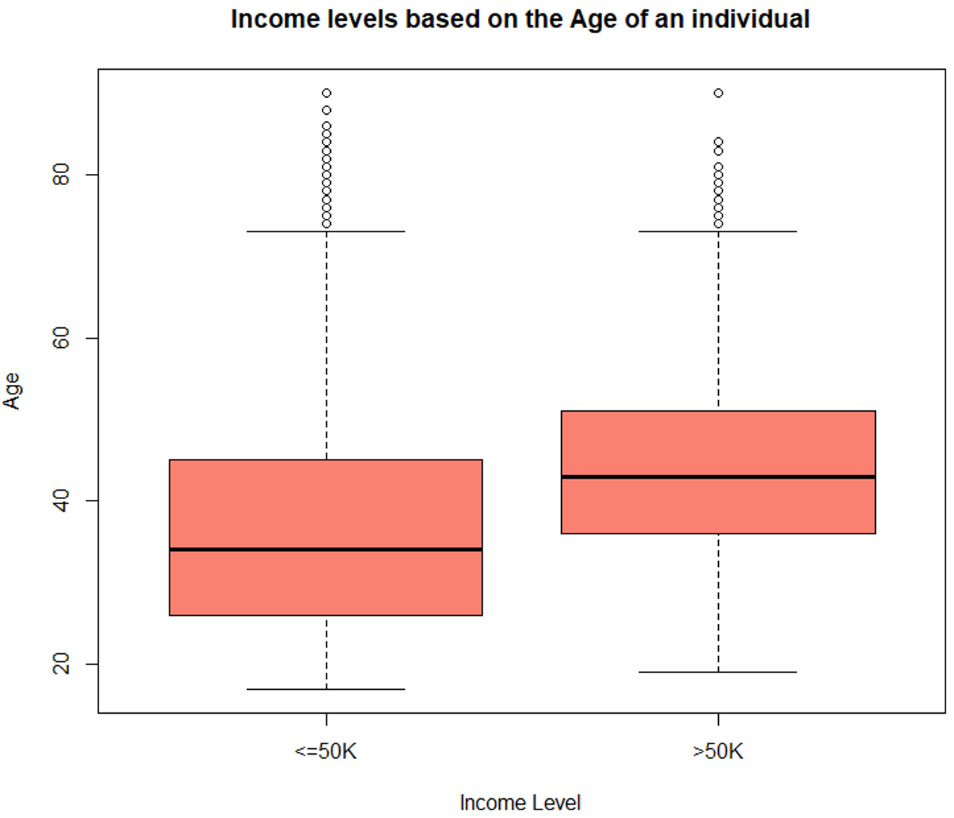
Box Plot – Data Science Projects – Edureka
#Histogram for age variable
incomeBelow50K = (TrainSet$incomelevel == "<=50K")
xlimit = c (min (TrainSet$age), max (TrainSet$age))
ylimit = c (0, 1600)

hist1 = qplot (age, data = TrainSet[incomeBelow50K,], margins = TRUE,
binwidth = 2, xlim = xlimit, ylim = ylimit, colour = incomelevel)

hist2 = qplot (age, data = TrainSet[!incomeBelow50K,], margins = TRUE,
binwidth = 2, xlim = xlimit, ylim = ylimit, colour = incomelevel)

grid.arrange (hist1, hist2, nrow = 2)
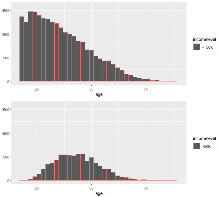
Histogram – Data Science Projects – Edureka
The above illustrations show that the age variable is varying with the level of income and hence it is a strong predictor variable.
This variable denotes the number of years of education of an individual. Let’s see how the ‘educationnum’ variable varies with respect to the income levels:
> summary (TrainSet$educationnum)
Min. 1st Qu. Median Mean 3rd Qu. Max.
1.00 9.00 10.00 10.12 13.00 16.00

#Boxplot for education-num variable
boxplot (educationnum ~ incomelevel, data = TrainSet,
main = "Years of Education distribution for different income levels",
xlab = "Income Levels", ylab = "Years of Education", col = "green")
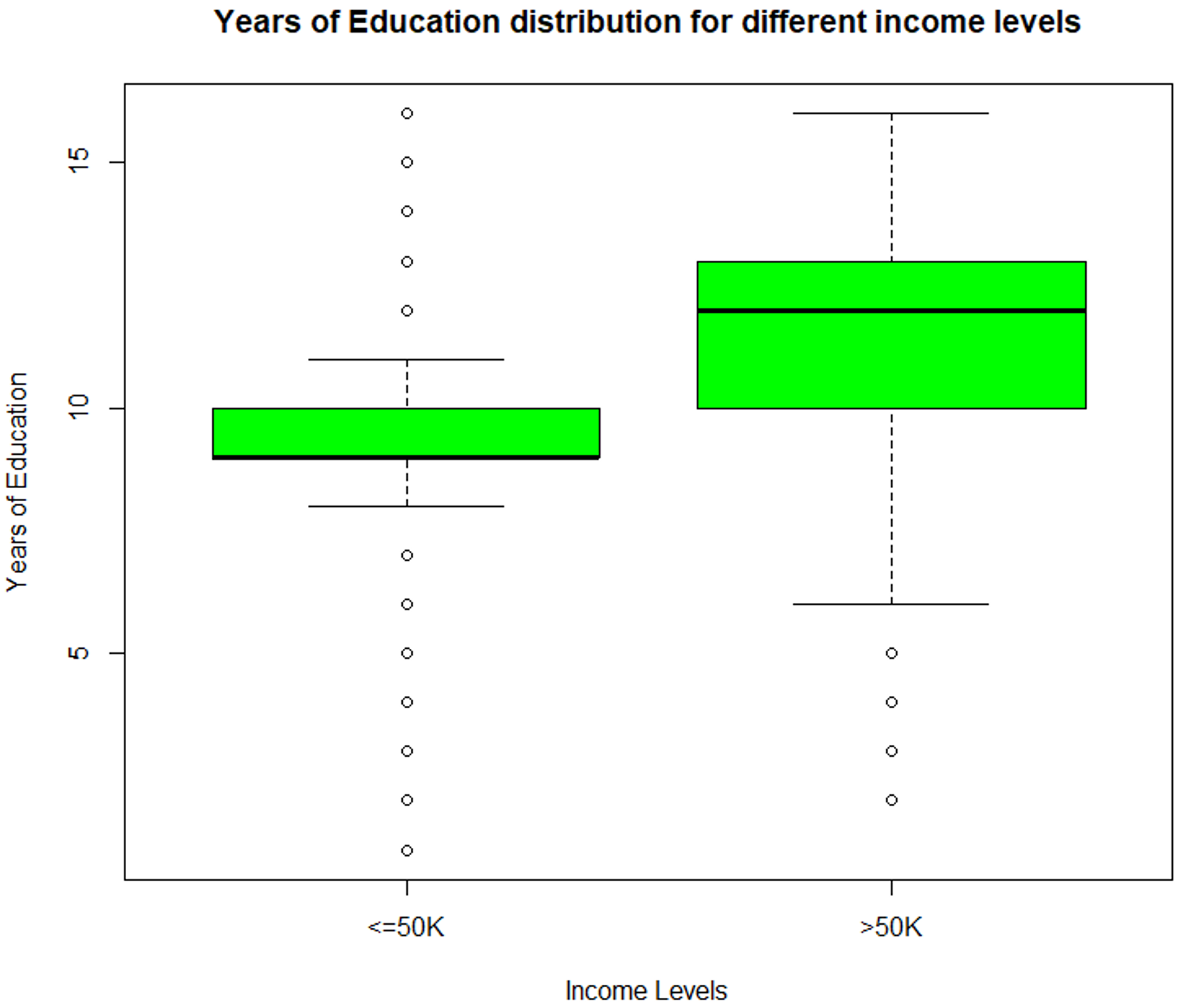
Data Exploration (educationnum) – Data Science Projects – Edureka
The above illustration depicts that the ‘educationnum’ variable varies for income levels <=50k and >50k, thus proving that it is a significant variable for predicting the outcome.
After studying the summary of the capital-gain and capital-loss variables for each income level, their means vary significantly, thus indicating that they are suitable variables for predicting an individual’s income level.
> summary (TrainSet[ TrainSet$incomelevel == "<=50K",
+                        c("capitalgain", "capitalloss")])
  capitalgain       capitalloss
 Min.   :    0.0   Min.   :   0.00
 1st Qu.:    0.0   1st Qu.:   0.00
 Median :    0.0   Median :   0.00
 Mean   :  148.9   Mean   :  53.45
 3rd Qu.:    0.0   3rd Qu.:   0.00
 Max.   :41310.0   Max.   :4356.00
Similarly, the ‘hoursperweek’ variable is evaluated to check if it is a significant predictor variable.
#Evaluate hours/week variable

> summary (TrainSet$hoursperweek)
Min. 1st Qu. Median Mean 3rd Qu. Max.
1.00 40.00 40.00 40.93 45.00 99.00

boxplot (hoursperweek ~ incomelevel, data = TrainSet,
main = "Hours Per Week distribution for different income levels",
xlab = "Income Levels", ylab = "Hours Per Week", col = "salmon")
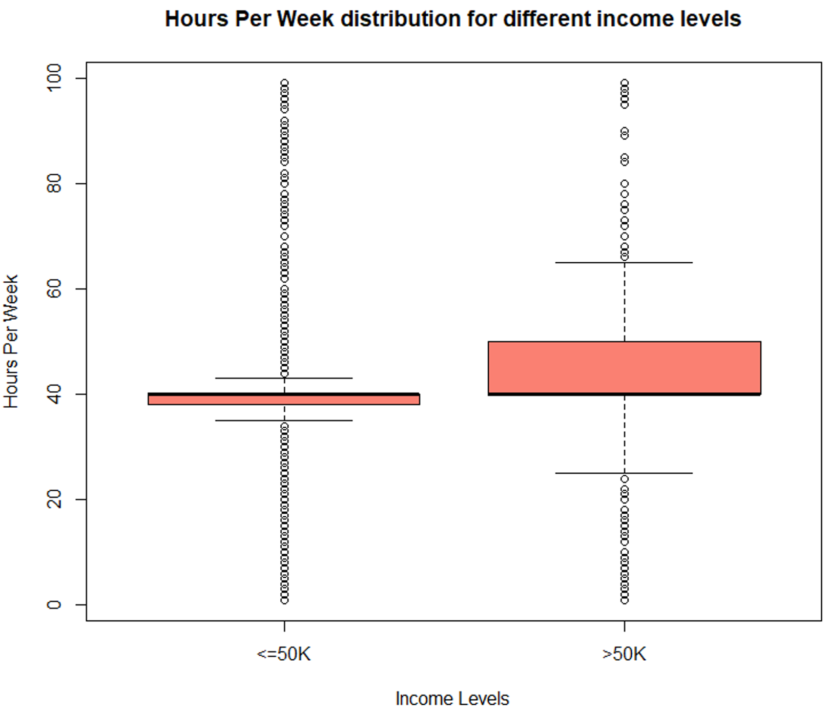
Data Exploration (hoursperweek) – Data Science Projects – Edureka
The boxplot shows a clear variation for different income levels which makes it an important variable for predicting the outcome.
Similarly, we’ll be evaluating categorical variables as well. In the below section I’ve created qplots for each variable and after evaluating the plots, it is clear that these variables are essential for predicting the income level of an individual.
Exploring work-class variable
#Evaluating work-class variable
qplot (incomelevel, data = TrainSet, fill = workclass) + facet_grid (. ~ workclass)

Data Exploration (workclass) – Data Science Projects – Edureka
#Evaluating occupation variable
qplot (incomelevel, data = TrainSet, fill = occupation) + facet_grid (. ~ occupation)
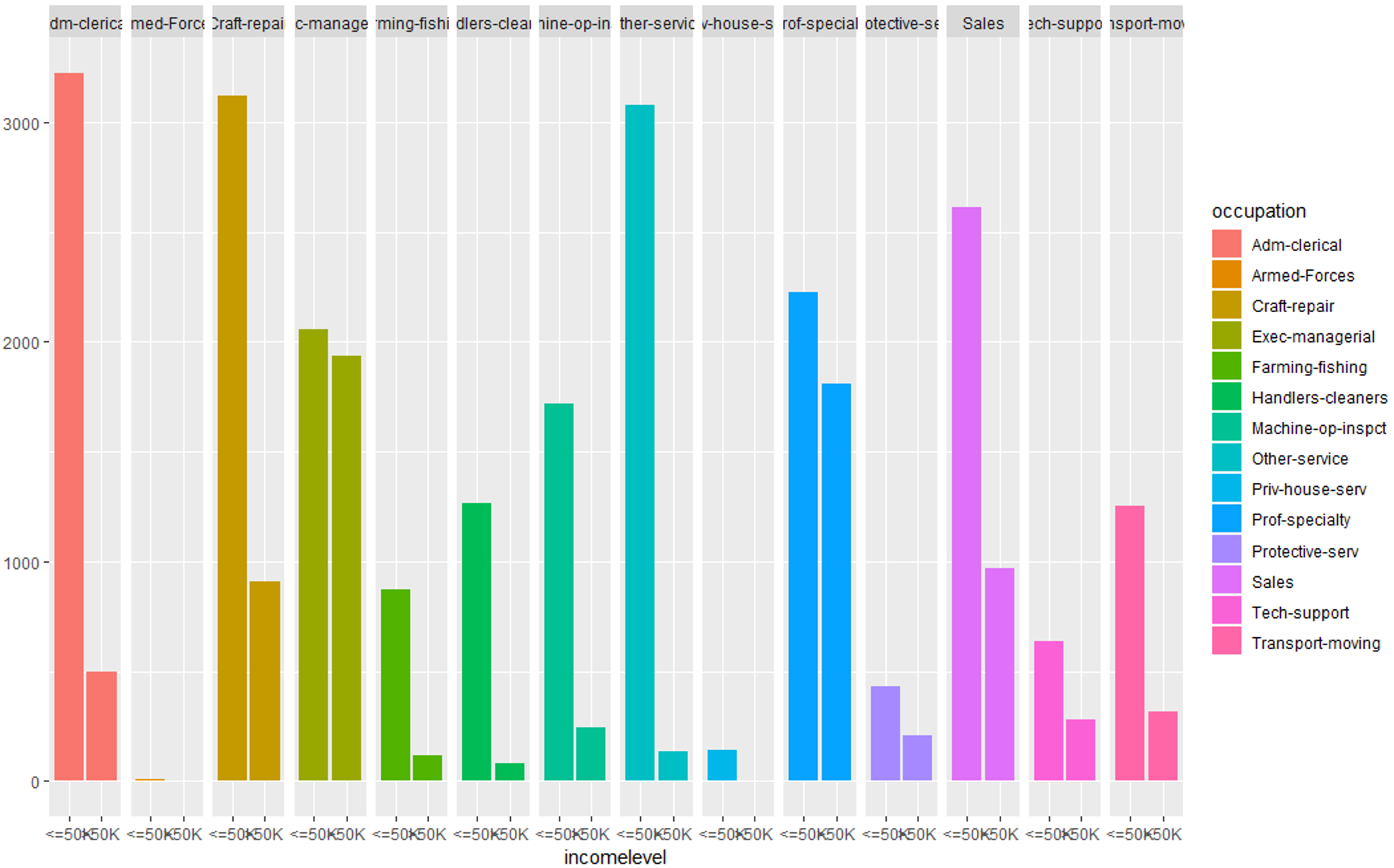
Data Exploration (occupation) – Data Science Projects – Edureka
#Evaluating marital-status variable
qplot (incomelevel, data = TrainSet, fill = maritalstatus) + facet_grid (. ~ maritalstatus)
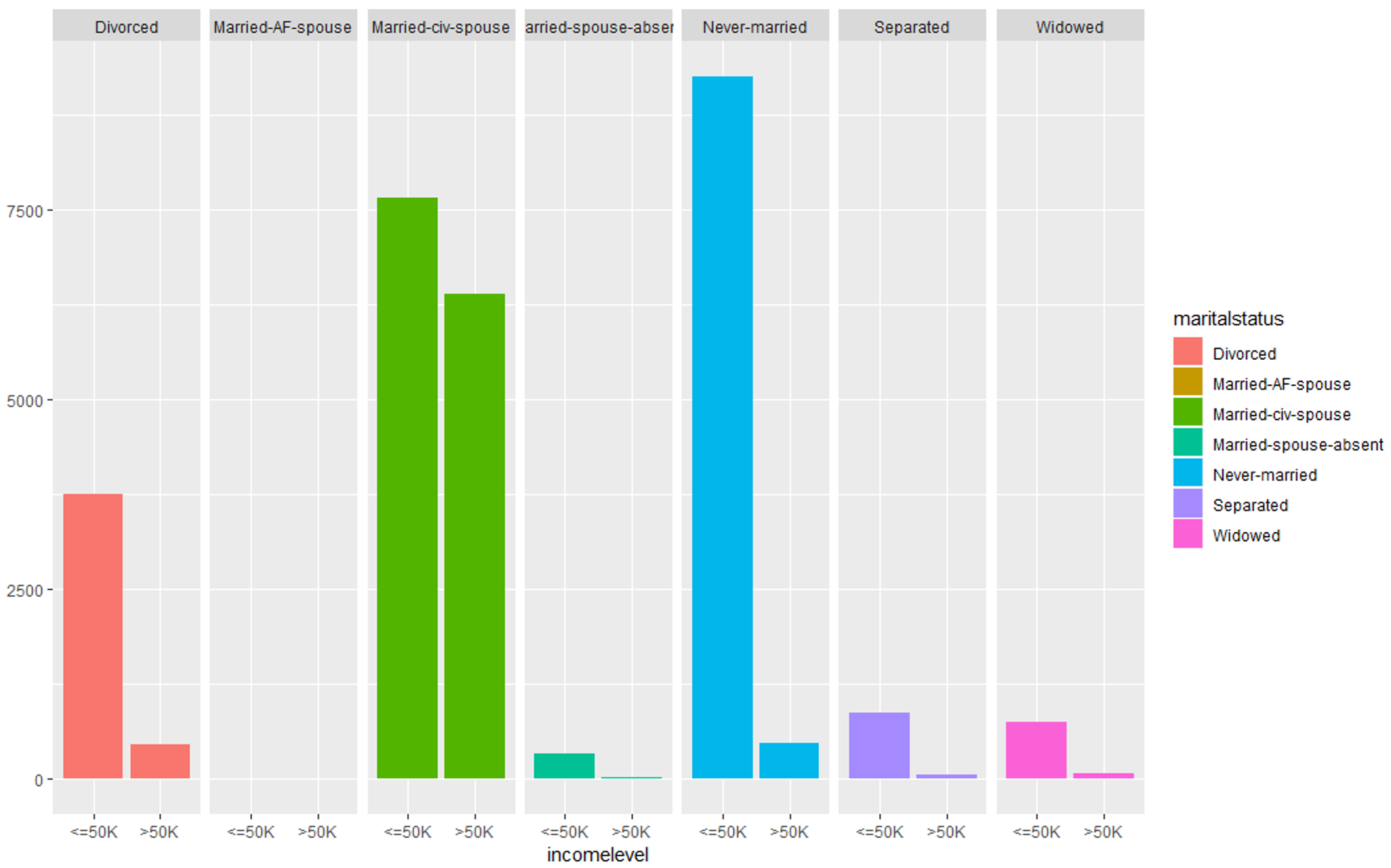
Data Exploration (martialstatus) – Data Science Projects – Edureka
#Evaluating relationship variable
qplot (incomelevel, data = TrainSet, fill = relationship) + facet_grid (. ~ relationship)
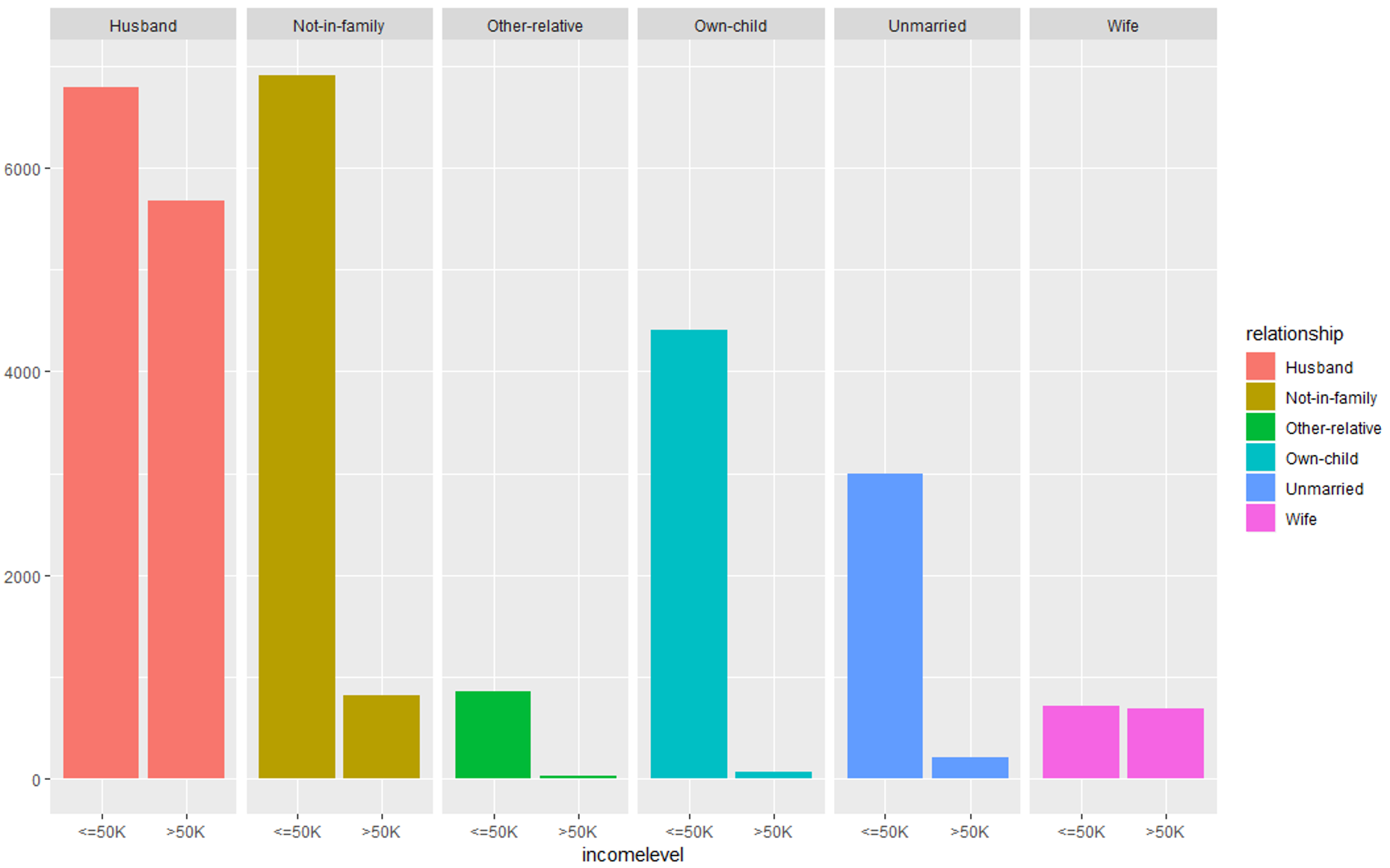
Data Exploration (relationship) – Data Science Projects – Edureka
All these graphs show that these set of predictor variables are significant for building our predictive model.
Step 4: Building A Model
So, after evaluating all our predictor variables, it is finally time to perform Predictive analytics. In this stage, we’ll build a predictive model that will predict whether an individual earns above USD 50,000 based on the predictor variables we evaluated in the previous section.
To build this model I’ve made use of the boosting algorithm since we have to classify an individual into either of the two classes, i.e:
Income level <= USD 50,000
Income level > USD 50,000
#Building the model
set.seed (32323)

trCtrl = trainControl(method = "cv", number = 10)

boostFit = train (incomelevel ~ age + workclass + education + educationnum +
maritalstatus + occupation + relationship +
race + capitalgain + capitalloss + hoursperweek +
nativecountry, trControl = trCtrl,
method = "gbm", data = TrainSet, verbose = FALSE)
Since we’re using an ensemble classification algorithm, I’ve also implemented the Cross-Validation technique to prevent overfitting of the model.
Step 5: Checking the accuracy of the model
To evaluate the accuracy of the model, we’re going to use a confusion matrix:
#Checking the accuracy of the model

> confusionMatrix (TrainSet$incomelevel, predict (boostFit, TrainSet))
Confusion Matrix and Statistics

Reference
Prediction <=50K >50K
<=50K 21404 1250 >50K 2927 4581

Accuracy : 0.8615
95% CI : (0.8576, 0.8654)
No Information Rate : 0.8067
P-Value [Acc > NIR] : < 2.2e-16

Kappa : 0.5998

Mcnemar's Test P-Value : < 2.2e-16

Sensitivity : 0.8797
Specificity : 0.7856
Pos Pred Value : 0.9448
Neg Pred Value : 0.6101
Prevalence : 0.8067
Detection Rate : 0.7096
Detection Prevalence : 0.7511
Balanced Accuracy : 0.8327

'Positive' Class : <=50K
The output shows that our model calculates the income level of an individual with an accuracy of approximately 86%, which is a good number.
So far, we used the training data set to build the model, now its time to validate the model by using the testing data set.
Step 5: Load and evaluate the test data set
Just like how we cleaned our training data set, our testing data must also be prepared in such a way that it does not have any null values or unnecessary predictor variables, only then can we use the test data to validate our model.
Start by loading the testing data set:
#Load the testing data set
testing = read.table (testFile, header = FALSE, sep = ",",
strip.white = TRUE, col.names = colNames,
na.strings = "?", fill = TRUE, stringsAsFactors = TRUE)
Next, we’re studying the structure of our data set.
#Display structure of the data
> str (testing)
'data.frame': 16282 obs. of 15 variables:
$ age : Factor w/ 74 levels "|1x3 Cross validator",..: 1 10 23 13 29 3 19 14 48 9 ...
$ workclass : Factor w/ 9 levels "","Federal-gov",..: 1 5 5 3 5 NA 5 NA 7 5 ...
$ fnlwgt : int NA 226802 89814 336951 160323 103497 198693 227026 104626 369667 ...
$ education : Factor w/ 17 levels "","10th","11th",..: 1 3 13 9 17 17 2 13 16 17 ...
$ educationnum : int NA 7 9 12 10 10 6 9 15 10 ...
$ maritalstatus: Factor w/ 8 levels "","Divorced",..: 1 6 4 4 4 6 6 6 4 6 ...
$ occupation : Factor w/ 15 levels "","Adm-clerical",..: 1 8 6 12 8 NA 9 NA 11 9 ...
$ relationship : Factor w/ 7 levels "","Husband","Not-in-family",..: 1 5 2 2 2 5 3 6 2 6 ...
$ race : Factor w/ 6 levels "","Amer-Indian-Eskimo",..: 1 4 6 6 4 6 6 4 6 6 ...
$ sex : Factor w/ 3 levels "","Female","Male": 1 3 3 3 3 2 3 3 3 2 ...
$ capitalgain : int NA 0 0 0 7688 0 0 0 3103 0 ...
$ capitalloss : int NA 0 0 0 0 0 0 0 0 0 ...
$ hoursperweek : int NA 40 50 40 40 30 30 40 32 40 ...
$ nativecountry: Factor w/ 41 levels "","Cambodia",..: 1 39 39 39 39 39 39 39 39 39 ...
$ incomelevel : Factor w/ 3 levels "","<=50K.",">50K.": 1 2 2 3 3 2 2 2 3 2 ...
In the below code snippet we’re looking for complete observations that do not have any null data or missing data.
> table (complete.cases (testing))
FALSE TRUE
1222 15060
> summary  (testing [!complete.cases(testing),])
      age                 workclass       fnlwgt               education    educationnum
 20     : 73   Private         :189   Min.   :  13862   Some-college:366   Min.   : 1.000
 19     : 71   Self-emp-not-inc: 24   1st Qu.: 116834   HS-grad     :340   1st Qu.: 9.000
 18     : 64   State-gov       : 16   Median : 174274   Bachelors   :144   Median :10.000
 21     : 62   Local-gov       : 10   Mean   : 187207   11th        : 66   Mean   : 9.581
 22     : 53   Federal-gov     :  9   3rd Qu.: 234791   10th        : 53   3rd Qu.:10.000
 17     : 35   (Other)         : 11   Max.   :1024535   Masters     : 47   Max.   :16.000
 (Other):864   NA's            :963   NA's   :1         (Other)     :206   NA's   :1
               maritalstatus           occupation          relationship                 race
 Never-married        :562   Prof-specialty : 62                 :  1                     :  1
 Married-civ-spouse   :413   Other-service  : 32   Husband       :320   Amer-Indian-Eskimo: 10
 Divorced             :107   Sales          : 30   Not-in-family :302   Asian-Pac-Islander: 72
 Widowed              : 75   Exec-managerial: 28   Other-relative: 65   Black             :150
 Separated            : 33   Craft-repair   : 23   Own-child     :353   Other             : 13
 Married-spouse-absent: 28   (Other)        : 81   Unmarried     :103   White             :976
 (Other)              :  4   NA's           :966   Wife          : 78
     sex       capitalgain       capitalloss       hoursperweek         nativecountry
       :  1   Min.   :    0.0   Min.   :   0.00   Min.   : 1.00   UnitedStates
 Female:508   1st Qu.:    0.0   1st Qu.:   0.00   1st Qu.:20.00   Mexico
              Mean   :  608.3   Mean   :  73.81   Mean   :33.49   South
              3rd Qu.:    0.0   3rd Qu.:   0.00   3rd Qu.:40.00   England
              Max.   :99999.0   Max.   :2603.00   Max.   :99.00   (Other)
              NA's   :1         NA's   :1         NA's   :1       NA's         :274
From the summary it is clear that we have many NA values in the ‘workclass’, ‘occupation’ and ‘nativecountry’ variables, so let’s get rid of these variables.
#Removing NAs
TestSet = testing [!is.na (testing$workclass) & !is.na (testing$occupation), ]
TestSet = TestSet [!is.na (TestSet$nativecountry), ]

#Removing unnecessary variables
TestSet$fnlwgt = NULL
Step 6: Validate the model
The test data set is applied to the predictive model to validate the efficiency of the model. The following code snippet shows how this is done:
#Testing model
TestSet$predicted = predict (boostFit, TestSet)
table(TestSet$incomelevel, TestSet$predicted)

actuals_preds <- data.frame(cbind(actuals=TestSet$incomelevel, predicted=TestSet$predicted)) # make actuals_predicteds dataframe.
correlation_accuracy <- cor(actuals_preds)
head(actuals_preds)
The table is used to compare the predicted values to the actual income levels of an individual. This model can further be improved by introducing some variations in the model or by using an alternate algorithm.
So, we just executed an entire Data Science Project from scratch.
In the below section I’ve compiled a set of projects that will help you gain experience in data cleaning, statistical analysis, data modeling, and data visualization.
Consider this as your homework.
Learn OpenAI’s cutting-edge technology which gives instant answers to every solutions with Edureka’s ChatGPT certification training course.
Data Science plays a huge role in forecasting sales and risks in the retail sector. Majority of the leading retail stores implement Data Science to keep a track of their customer needs and make better business decisions. Walmart is one such retailer.
Problem Statement: To analyze the Walmart Sales Data set in order to predict department-wise sales for each of their stores.
Data Set Description: The data set used for this project contains historical training data, which covers sales details from 2010-02-05 to 2012-11-01. For the analysis of this problem, the following predictor variables are used:
By studying the dependency of these predictor variables on the response variable, you can predict or forecast sales for the upcoming months.
Logic:
With the increase in the number of crimes taking place in Chicago, law enforcement agencies are trying their best to understand the reason behind such actions. Analyses like these can not only help understand the reasons behind these crimes, but they can also prevent further crimes.
Problem Statement: To analyze and explore the Chicago Crime data set to understand trends and patterns that will help predict any future occurrences of such felonies.
Data Set Description: The dataset used for this project consists of every reported instance of a crime in the city of Chicago from 01/01/2014 to 10/24/2016.
For this analysis, the data set contains many predictor variables such as:
Logic:
Like any other Data Science project, the below-described series of steps are followed:
Import the Data Set: The data set needed for this project can be downloaded from Kaggle.
Data Cleaning: In this stage, you must make sure to get rid of all inconsistencies, such as missing values and any redundant variables.
Data Exploration: You can begin this stage by translating the occurrence of crimes into plots on a geographical map of the city. Graphically studying each predictor variable will help you understand which variables are essential for building the model.
Data Modelling: For this particular problem statement, since the nature of crimes varies, it is reasonable to build a clustering model. K-means is the most suitable algorithm for this analysis since it is easy to build clusters using k-means.
Analyzing patterns: Since this problem statement requires you to draw patterns and insights about the crimes, this step mainly involves creating reports and drawing conclusions from the data model.
Validate the model: At this stage, you should evaluate the efficiency of the data model by using the testing data set and finally calculate the accuracy of the model by using a confusion matrix.
Every successful Data Scientist has built at least one recommendation engine in his career. Personalized Recommendation engines are regarded as the holy grails of Data Science projects and that’s why I’ve added this project in the blog.
Problem Statement: To analyze the Movie Lens data set in order to understand trends and patterns that will help to recommend new movies to users.
Data Set Description: The data set used for this project was collected by the GroupLens Research Project at the University of Minnesota.
The dataset consists of the following predictor variables:
By studying these predictor variables, a model can be built for recommending movies to users.
Logic:
Having a Text Mining project in your resume will definitely increase your chances of getting hired as a Data Scientist. It involves advanced analytics and data mining that will make you a skilled Data Scientist. A popular application of text mining is sentiment analysis, which is extremely useful in social media monitoring because it helps to gain an overview of the wider public opinion on certain topics.
Problem Statement: To perform pre-processing, text analysis, text mining and visualization on a set of documents using Natural Language Processing techniques.
Data Set Description: This data set contains scripts of the famous Star Wars Series from the Original Trilogy Episodes i.e., IV, V and VI.
Logic:
So these were a few Projects on Data Science to get you started. I’ve provided you with the blueprint to solve each of these use cases, all you have to do is follow the steps. Don’t hesitate if you want to experiment and do your own thing.
Also, don’t forget to share your implementation in the comment section, I would love to know how your solution turned out.
Now that you know how to solve a real-world problem by using Data Science, I’m sure you’re curious to learn more. Here’s a list of blogs that will help you get started:
With this, we come to the end of this blog. If you have any queries regarding this topic, please leave a comment below and we’ll get back to you.
Stay tuned for more blogs on trending technologies.
The need for Data Science with Python programming professionals has increased dramatically, making Data Science with Python courses ideal for people at all levels of expertise. The Data Science with Python Course is ideal for professionals in analytics looking to work in conjunction with Python, Software, and IT professionals interested in the area of Analytics and anyone with a passion for Data Science.
Also, If you are looking for online structured training in Data Science, edureka! has a specially curated Data Science Course that helps you gain expertise in Statistics, Data Wrangling, Exploratory Data Analysis, and Machine Learning Algorithms like K-Means Clustering, Decision Trees, Random Forest, and Naive Bayes. You’ll also learn the concepts of Time Series, Text Mining, and an introduction to Deep Learning. New batches for this course are starting soon!!


 Thank you for registering Join Edureka Meetup community for 100+ Free Webinars each month JOIN MEETUP GROUP