

Advanced Certification in Agentic AI Engineer ...
- 67k Enrolled Learners
- Weekend
- Live Class
(45931)


 Copy Link!
In this blog, let us discuss what is Convolutional Neural Network (CNN) and the architecture behind Convolutional Neural Networks – which are designed to address image recognition systems and classification problems. Convolutional Neural Networks have wide applications in image and video recognition, recommendation systems and natural language processing.
We will be checking out the following concepts:
🐍 Ready to Unleash the Power of Python? Sign Up and get Edureka’s Comprehensive Online Python Course With Certificate with access to hundreds of Python learning Modules and 24/7 technical support.
Consider this image of the New York skyline, upon first glance you will see a lot of buildings and colors. So how does the computer process this image?

The image is broken down into 3 color-channels which is Red, Green and Blue. Each of these color channels are mapped to the image’s pixel.
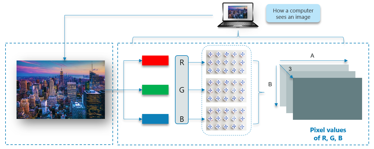
Then, the computer recognizes the value associated with each pixel and determine the size of the image.
However, for black-white images, there is only one channel and the concept is the same.
We cannot make use of fully connected networks when it comes to Convolutional Neural Networks, here’s why!
Consider the following image: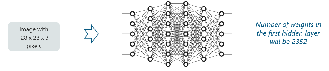
Here, we have considered an input of images with the size 28x28x3 pixels. If we input this to our Convolutional Neural Network, we will have about 2352 weights in the first hidden layer itself.
But this case isn’t practical. Now, take a look at this:
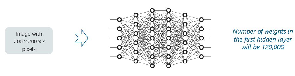
Any generic input image will atleast have 200x200x3 pixels in size. The size of the first hidden layer becomes a whooping 120,000. If this is just the first hidden layer, imagine the number of neurons needed to process an entire complex image-set.
This leads to over-fitting and isn’t practical. Hence, we cannot make use of fully connected networks.
Convolutional Neural Networks, like neural networks, are made up of neurons with learnable weights and biases. Each neuron receives several inputs, takes a weighted sum over them, pass it through an activation function and responds with an output.
The whole network has a loss function and all the tips and tricks that we developed for neural networks still apply on Convolutional Neural Networks.
Pretty straightforward, right?
Neural networks, as its name suggests, is a machine learning technique which is modeled after the brain structure. It comprises of a network of learning units called neurons.
These neurons learn how to convert input signals (e.g. picture of a cat) into corresponding output signals (e.g. the label “cat”), forming the basis of automated recognition.
Let’s take the example of automatic image recognition. The process of determining whether a picture contains a cat involves an activation function. If the picture resembles prior cat images the neurons have seen before, the label “cat” would be activated.
Hence, the more labeled images the neurons are exposed to, the better it learns how to recognize other unlabelled images. We call this the process of training neurons.
The intelligence of neural networks is uncanny. While artificial neural networks were researched as early in 1960s by Rosenblatt, it was only in late 2000s when deep learning using neural networks took off. The key enabler was the scale of computation power and datasets with Google pioneering research into deep learning. In July 2012, researchers at Google exposed an advanced neural network to a series of unlabelled, static images sliced from YouTube videos.
To their surprise, they discovered that the neural network learned a cat-detecting neuron on its own, supporting the popular assertion that “the internet is made of cats”.

There are four layered concepts we should understand in Convolutional Neural Networks:
Let’s begin by checking out a simple example:
Consider the image below:

Here, there are multiple renditions of X and O’s. This makes it tricky for the computer to recognize. But the goal is that if the input signal looks like previous images it has seen before, the “image” reference signal will be mixed into, or convolved with, the input signal. The resulting output signal is then passed on to the next layer.

So, the computer understands every pixel. In this case, the white pixels are said to be -1 while the black ones are 1. This is just the way we’ve implemented to differentiate the pixels in a basic binary classification.

Now if we would just normally search and compare the values between a normal image and another ‘x’ rendition, we would get a lot of missing pixels.
So, how do we fix this?

We take small patches of the pixels called filters and try to match them in the corresponding nearby locations to see if we get a match. By doing this, the Convolutional Neural Network gets a lot better at seeing similarity than directly trying to match the entire image.
Convolution has the nice property of being translational invariant. Intuitively, this means that each convolution filter represents a feature of interest (e.g pixels in letters) and the Convolutional Neural Network algorithm learns which features comprise the resulting reference (i.e. alphabet).
We have 4 steps for convolution:


Consider the above image – As you can see, we are done with the first 2 steps. We considered a feature image and one pixel from it. We multiplied this with the existing image and the product is stored in another buffer feature image.
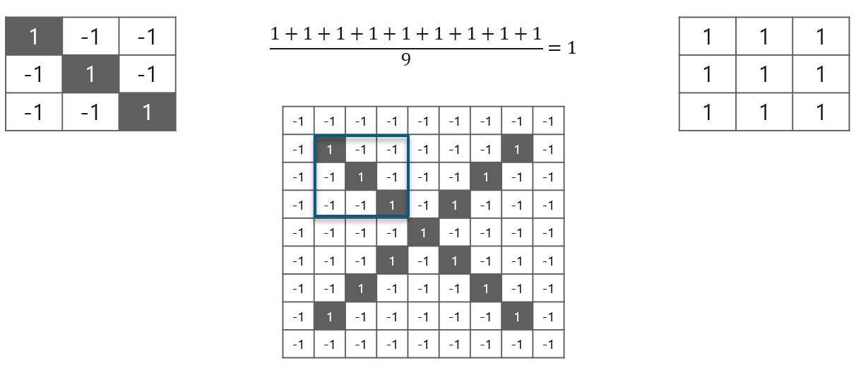
With this image, we completed the last 2 steps. We added the values which led to the sum. We then, divide this number by the total number of pixels in the feature image. When that is done, the final value obtained is placed at the center of the filtered image as shown below:

Now, we can move this filter around and do the same at any pixel in the image. For better clarity, let’s consider another example:

As you can see, here after performing the first 4 steps we have the value at 0.55! We take this value and place it in the image as explained before. This is done in the following image:

Similarly, we move the feature to every other position in the image and see how the feature matches that area. So after doing this, we will get the output as:

Here we considered just one filter. Similarly, we will perform the same convolution with every other filter to get the convolution of that filter.
The output signal strength is not dependent on where the features are located, but simply whether the features are present. Hence, an alphabet could be sitting in different positions and the Convolutional Neural Network algorithm would still be able to recognize it.
ReLU is an activation function. But, what is an activation function?
Rectified Linear Unit (ReLU) transform function only activates a node if the input is above a certain quantity, while the input is below zero, the output is zero, but when the input rises above a certain threshold, it has a linear relationship with the dependent variable.
Consider the below example:

We have considered a simple function with the values as mentioned above. So the function only performs an operation if that value is obtained by the dependent variable. For this example, the following values are obtained:

Why do we require ReLU here?

The main aim is to remove all the negative values from the convolution. All the positive values remain the same but all the negative values get changed to zero as shown below:

So after we process this particular feature we get the following output:

Now, similarly we do the same process to all the other feature images as well:

Inputs from the convolution layer can be “smoothened” to reduce the sensitivity of the filters to noise and variations. This smoothing process is called subsampling and can be achieved by taking averages or taking the maximum over a sample of the signal.
In this layer we shrink the image stack into a smaller size. Pooling is done after passing through the activation layer. We do this by implementing the following 4 steps:
Let us understand this with an example. Consider performing pooling with a window size of 2 and stride being 2 as well.

So in this case, we took window size to be 2 and we got 4 values to choose from. From those 4 values, the maximum value there is 1 so we pick 1. Also, note that we started out with a 7×7 matrix but now the same matrix after pooling came down to 4×4.
But we need to move the window across the entire image. The procedure is exactly as same as above and we need to repeat that for the entire image.

Do note that this is for one filter. We need to do it for 2 other filters as well. This is done and we arrive at the following result:
Well the easy part of this process is over. Next up, we need to stack up all these layers!
So to get the time-frame in one picture we’re here with a 4×4 matrix from a 7×7 matrix after passing the input through 3 layers – Convolution, ReLU and Pooling as shown below:

But can we further reduce the image from 4×4 to something lesser?
Yes, we can! We need to perform the 3 operations in an iteration after the first pass. So after the second pass we arrive at a 2×2 matrix as shown below:

The last layers in the network are fully connected, meaning that neurons of preceding layers are connected to every neuron in subsequent layers.
This mimics high level reasoning where all possible pathways from the input to output are considered.
Also, fully connected layer is the final layer where the classification actually happens. Here we take our filtered and shrinked images and put them into one single list as shown below:
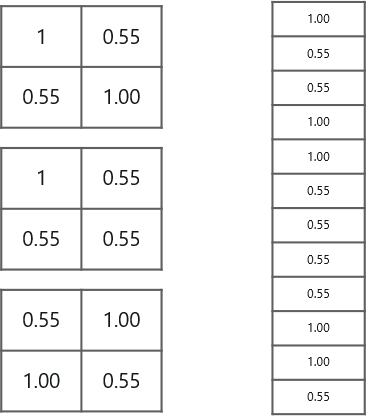
So next, when we feed in, ‘X’ and ‘O’ there will be some element in the vector that will be high. Consider the image below, as you can see for ‘X’ there are different elements that are high and similarly, for ‘O’ we have different elements that are high:
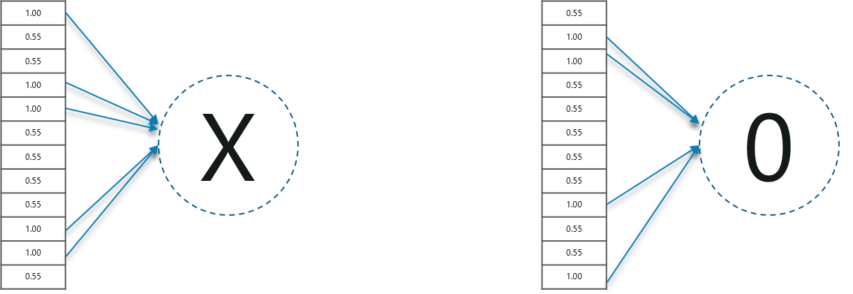
Well, what did we understand from the above image?
When the 1st, 4th, 5th, 10th and 11th values are high, we can classify the image as ‘x’. The concept is similar for the other alphabets as well – when certain values are arranged the way they are, they can be mapped to an actual letter or a number which we require, simple right?
At this point in time, we’re done training the network and we can begin to predict and check the working of the classifier. Let’s check out a simple example:

In the above image, we have a 12 element vector obtained after passing the input of a random letter through all the layers of our network.
But, how do we check to know what we’ve obtained is right or wrong?
We make predictions based on the output data by comparing the obtained values with list of ‘x’and ‘o’!

Well, it is really easy. We just added the values we which found out as high (1st, 4th, 5th, 10th and 11th) from the vector table of X and we got the sum to be 5. We did the exact same thing with the input image and got a value of 4.56.
When we divide the value we have a probability match to be 0.91! Let’s do the same with the vector table of ‘o’ now:

We have the output as 0.51 with this table. Well, probability being 0.51 is less than 0.91, isn’t it?
So we can conclude that the resulting input image is an ‘x’!
Let’s train a network to classify images from the CIFAR10 Dataset using a Convolution Neural Network built in TensorFlow.
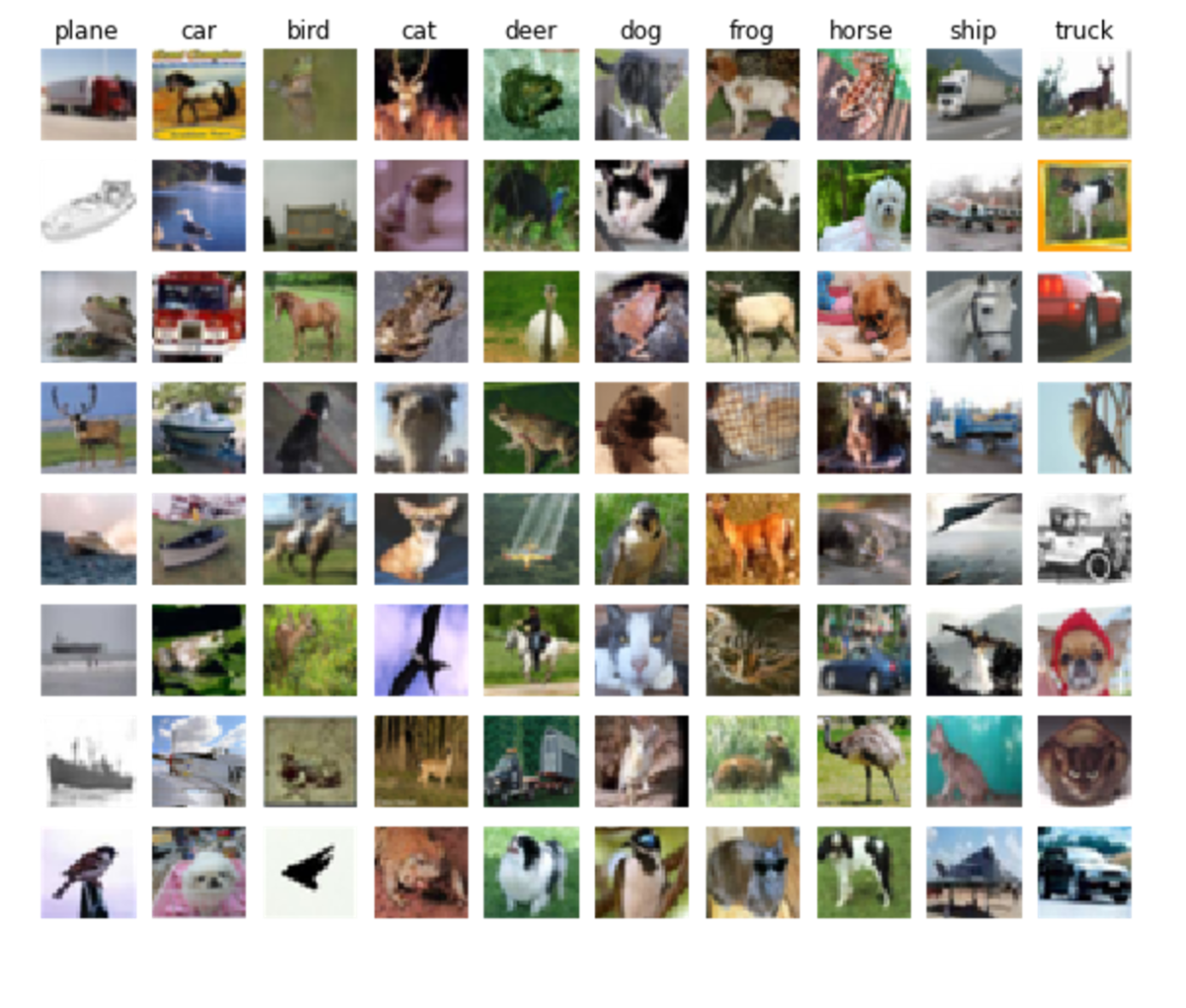
Consider the following Flowchart to understand the working of the use-case:

Install Necessary Packages:
pip3 install numpy tensorflow pickleTrain The Network:
import numpy as np
import tensorflow as tf
from time import time
import math


from include.data import get_data_set
from include.model import model, lr


train_x, train_y = get_data_set("train")
test_x, test_y = get_data_set("test")
tf.set_random_seed(21)
x, y, output, y_pred_cls, global_step, learning_rate = model()
global_accuracy = 0
epoch_start = 0


# PARAMS
_BATCH_SIZE = 128
_EPOCH = 60
_SAVE_PATH = "./tensorboard/cifar-10-v1.0.0/"


# LOSS AND OPTIMIZER
loss = tf.reduce_mean(tf.nn.softmax_cross_entropy_with_logits_v2(logits=output, labels=y))
optimizer = tf.train.AdamOptimizer(learning_rate=learning_rate,
                                   beta1=0.9,
                                   beta2=0.999,
                                   epsilon=1e-08).minimize(loss, global_step=global_step)


# PREDICTION AND ACCURACY CALCULATION
correct_prediction = tf.equal(y_pred_cls, tf.argmax(y, axis=1))
accuracy = tf.reduce_mean(tf.cast(correct_prediction, tf.float32))


# SAVER
merged = tf.summary.merge_all()
saver = tf.train.Saver()
sess = tf.Session()
train_writer = tf.summary.FileWriter(_SAVE_PATH, sess.graph)


try:
    print("
Trying to restore last checkpoint ...")
    last_chk_path = tf.train.latest_checkpoint(checkpoint_dir=_SAVE_PATH)
    saver.restore(sess, save_path=last_chk_path)
    print("Restored checkpoint from:", last_chk_path)
except ValueError:
    print("
Failed to restore checkpoint. Initializing variables instead.")
    sess.run(tf.global_variables_initializer())


def train(epoch):
    global epoch_start
    epoch_start = time()
    batch_size = int(math.ceil(len(train_x) / _BATCH_SIZE))
    i_global = 0

    for s in range(batch_size):
        batch_xs = train_x[s*_BATCH_SIZE: (s+1)*_BATCH_SIZE]
        batch_ys = train_y[s*_BATCH_SIZE: (s+1)*_BATCH_SIZE]

        start_time = time()
        i_global, _, batch_loss, batch_acc = sess.run(
            [global_step, optimizer, loss, accuracy],
            feed_dict={x: batch_xs, y: batch_ys, learning_rate: lr(epoch)})
        duration = time() - start_time

        if s % 10 == 0:
            percentage = int(round((s/batch_size)*100))

            bar_len = 29
            filled_len = int((bar_len*int(percentage))/100)
            bar = '=' * filled_len + '>' + '-' * (bar_len - filled_len)

            msg = "Global step: {:>5} - [{}] {:>3}% - acc: {:.4f} - loss: {:.4f} - {:.1f} sample/sec"
            print(msg.format(i_global, bar, percentage, batch_acc, batch_loss, _BATCH_SIZE / duration))

    test_and_save(i_global, epoch)


def test_and_save(_global_step, epoch):
    global global_accuracy
    global epoch_start

    i = 0
    predicted_class = np.zeros(shape=len(test_x), dtype=np.int)
    while i < len(test_x): j = min(i + _BATCH_SIZE, len(test_x)) batch_xs = test_x[i:j, :] batch_ys = test_y[i:j, :] predicted_class[i:j] = sess.run( y_pred_cls, feed_dict={x: batch_xs, y: batch_ys, learning_rate: lr(epoch)} ) i = j correct = (np.argmax(test_y, axis=1) == predicted_class) acc = correct.mean()*100 correct_numbers = correct.sum() hours, rem = divmod(time() - epoch_start, 3600) minutes, seconds = divmod(rem, 60) mes = " Epoch {} - accuracy: {:.2f}% ({}/{}) - time: {:0>2}:{:0>2}:{:05.2f}"
    print(mes.format((epoch+1), acc, correct_numbers, len(test_x), int(hours), int(minutes), seconds))

    if global_accuracy != 0 and global_accuracy < acc: summary = tf.Summary(value=[ tf.Summary.Value(tag="Accuracy/test", simple_value=acc), ]) train_writer.add_summary(summary, _global_step) saver.save(sess, save_path=_SAVE_PATH, global_step=_global_step) mes = "This epoch receive better accuracy: {:.2f} > {:.2f}. Saving session..."
        print(mes.format(acc, global_accuracy))
        global_accuracy = acc

    elif global_accuracy == 0:
        global_accuracy = acc

    print("###########################################################################################################")


def main():
    train_start = time()

    for i in range(_EPOCH):
        print("
Epoch: {}/{}
".format((i+1), _EPOCH))
        train(i)

    hours, rem = divmod(time() - train_start, 3600)
    minutes, seconds = divmod(rem, 60)
    mes = "Best accuracy pre session: {:.2f}, time: {:0>2}:{:0>2}:{:05.2f}"
    print(mes.format(global_accuracy, int(hours), int(minutes), seconds))


if __name__ == "__main__":
    main()


sess.close()
Output:
Epoch: 60/60

Global step: 23070 - [>-----------------------------]   0% - acc: 0.9531 - loss: 1.5081 - 7045.4 sample/sec
Global step: 23080 - [>-----------------------------]   3% - acc: 0.9453 - loss: 1.5159 - 7147.6 sample/sec
Global step: 23090 - [=>----------------------------]   5% - acc: 0.9844 - loss: 1.4764 - 7154.6 sample/sec
Global step: 23100 - [==>---------------------------]   8% - acc: 0.9297 - loss: 1.5307 - 7104.4 sample/sec
Global step: 23110 - [==>---------------------------]  10% - acc: 0.9141 - loss: 1.5462 - 7091.4 sample/sec
Global step: 23120 - [===>--------------------------]  13% - acc: 0.9297 - loss: 1.5314 - 7162.9 sample/sec
Global step: 23130 - [====>-------------------------]  15% - acc: 0.9297 - loss: 1.5307 - 7174.8 sample/sec
Global step: 23140 - [=====>------------------------]  18% - acc: 0.9375 - loss: 1.5231 - 7140.0 sample/sec
Global step: 23150 - [=====>------------------------]  20% - acc: 0.9297 - loss: 1.5301 - 7152.8 sample/sec
Global step: 23160 - [======>-----------------------]  23% - acc: 0.9531 - loss: 1.5080 - 7112.3 sample/sec
Global step: 23170 - [=======>----------------------]  26% - acc: 0.9609 - loss: 1.5000 - 7154.0 sample/sec
Global step: 23180 - [========>---------------------]  28% - acc: 0.9531 - loss: 1.5074 - 6862.2 sample/sec
Global step: 23190 - [========>---------------------]  31% - acc: 0.9609 - loss: 1.4993 - 7134.5 sample/sec
Global step: 23200 - [=========>--------------------]  33% - acc: 0.9609 - loss: 1.4995 - 7166.0 sample/sec
Global step: 23210 - [==========>-------------------]  36% - acc: 0.9375 - loss: 1.5231 - 7116.7 sample/sec
Global step: 23220 - [===========>------------------]  38% - acc: 0.9453 - loss: 1.5153 - 7134.1 sample/sec
Global step: 23230 - [===========>------------------]  41% - acc: 0.9375 - loss: 1.5233 - 7074.5 sample/sec
Global step: 23240 - [============>-----------------]  43% - acc: 0.9219 - loss: 1.5387 - 7176.9 sample/sec
Global step: 23250 - [=============>----------------]  46% - acc: 0.8828 - loss: 1.5769 - 7144.1 sample/sec
Global step: 23260 - [==============>---------------]  49% - acc: 0.9219 - loss: 1.5383 - 7059.7 sample/sec
Global step: 23270 - [==============>---------------]  51% - acc: 0.8984 - loss: 1.5618 - 6638.6 sample/sec
Global step: 23280 - [===============>--------------]  54% - acc: 0.9453 - loss: 1.5151 - 7035.7 sample/sec
Global step: 23290 - [================>-------------]  56% - acc: 0.9609 - loss: 1.4996 - 7129.0 sample/sec
Global step: 23300 - [=================>------------]  59% - acc: 0.9609 - loss: 1.4997 - 7075.4 sample/sec
Global step: 23310 - [=================>------------]  61% - acc: 0.8750 - loss: 1.5842 - 7117.8 sample/sec
Global step: 23320 - [==================>-----------]  64% - acc: 0.9141 - loss: 1.5463 - 7157.2 sample/sec
Global step: 23330 - [===================>----------]  66% - acc: 0.9062 - loss: 1.5549 - 7169.3 sample/sec
Global step: 23340 - [====================>---------]  69% - acc: 0.9219 - loss: 1.5389 - 7164.4 sample/sec
Global step: 23350 - [====================>---------]  72% - acc: 0.9609 - loss: 1.5002 - 7135.4 sample/sec
Global step: 23360 - [=====================>--------]  74% - acc: 0.9766 - loss: 1.4842 - 7124.2 sample/sec
Global step: 23370 - [======================>-------]  77% - acc: 0.9375 - loss: 1.5231 - 7168.5 sample/sec
Global step: 23380 - [======================>-------]  79% - acc: 0.8906 - loss: 1.5695 - 7175.2 sample/sec
Global step: 23390 - [=======================>------]  82% - acc: 0.9375 - loss: 1.5225 - 7132.1 sample/sec
Global step: 23400 - [========================>-----]  84% - acc: 0.9844 - loss: 1.4768 - 7100.1 sample/sec
Global step: 23410 - [=========================>----]  87% - acc: 0.9766 - loss: 1.4840 - 7172.0 sample/sec
Global step: 23420 - [==========================>---]  90% - acc: 0.9062 - loss: 1.5542 - 7122.1 sample/sec
Global step: 23430 - [==========================>---]  92% - acc: 0.9297 - loss: 1.5313 - 7145.3 sample/sec
Global step: 23440 - [===========================>--]  95% - acc: 0.9297 - loss: 1.5301 - 7133.3 sample/sec
Global step: 23450 - [============================>-]  97% - acc: 0.9375 - loss: 1.5231 - 7135.7 sample/sec
Global step: 23460 - [=============================>] 100% - acc: 0.9250 - loss: 1.5362 - 10297.5 sample/sec

Epoch 60 - accuracy: 78.81% (7881/10000)
This epoch receive better accuracy: 78.81 > 78.78. Saving session...
###########################################################################################################
Run Network on Test DataSet:
import numpy as np
import tensorflow as tf

from include.data import get_data_set
from include.model import model


test_x, test_y = get_data_set("test")
x, y, output, y_pred_cls, global_step, learning_rate = model()


_BATCH_SIZE = 128
_CLASS_SIZE = 10
_SAVE_PATH = "./tensorboard/cifar-10-v1.0.0/"


saver = tf.train.Saver()
sess = tf.Session()


try:
    print("
Trying to restore last checkpoint ...")
    last_chk_path = tf.train.latest_checkpoint(checkpoint_dir=_SAVE_PATH)
    saver.restore(sess, save_path=last_chk_path)
    print("Restored checkpoint from:", last_chk_path)
except ValueError:
    print("
Failed to restore checkpoint. Initializing variables instead.")
    sess.run(tf.global_variables_initializer())


def main():
    i = 0
    predicted_class = np.zeros(shape=len(test_x), dtype=np.int)
    while i < len(test_x):
        j = min(i + _BATCH_SIZE, len(test_x))
        batch_xs = test_x[i:j, :]
        batch_ys = test_y[i:j, :]
        predicted_class[i:j] = sess.run(y_pred_cls, feed_dict={x: batch_xs, y: batch_ys})
        i = j

    correct = (np.argmax(test_y, axis=1) == predicted_class)
    acc = correct.mean() * 100
    correct_numbers = correct.sum()
    print()
    print("Accuracy on Test-Set: {0:.2f}% ({1} / {2})".format(acc, correct_numbers, len(test_x)))


if __name__ == "__main__":
    main()


sess.close()
Simple output:
Trying to restore last checkpoint ...
Restored checkpoint from: ./tensorboard/cifar-10-v1.0.0/-23460

Accuracy on Test-Set: 78.81% (7881 / 10000)
Training Time
Here you can see how much time takes 60 epoch:
| Device | Batch Size | Time | Accuracy [%] |
| NVidia GTX 1070 | 128 | 8m 4s | 79.12 |
| Intel i7 7700HQ | 128 | 3h 30m | 78.91 |
Convolutional Neural Networks is a popular deep learning technique for current visual recognition tasks. Like all deep learning techniques, Convolutional Neural Networks are very dependent on the size and quality of the training data.
Given a well-prepared dataset, Convolutional Neural Networks are capable of surpassing humans at visual recognition tasks. However, they are still not robust to visual artifacts such as glare and noise, which humans are able to cope.
The theory of Convolutional Neural Networks is still being developed and researchers are working to endow it with properties such as active attention and online memory, allowing Convolutional Neural Networks to evaluate new items that are vastly different from what they were trained on.
This better emulates the mammalian visual system, thus moving towards a smarter artificial visual recognition system.
After reading this blog on Convolutional Neural Networks, I am pretty sure you want to know more about Deep Learning and Neural Networks. To know more about Deep Learning and Neural Networks you can refer the following blogs:
Convolutional Neural Network (CNN) | Edureka
This video will help you in understanding what is Convolutional Neural Network and how it works. It also includes a use-case, in which we will be creating a classifier using TensorFlow.


 Thank you for registering Join Edureka Meetup community for 100+ Free Webinars each month JOIN MEETUP GROUP


Very good critical for the beginners