How To Implement Classification In Machine Learning?

Classification in machine learning and statistics is a supervised learning approach in which the computer program learns from the data given to it and makes new observations or classifications. In this article, we will learn about classification in machine learning in detail.

The following topics are covered in this blog:

• What is Classification in Machine Learning?
• Classification Terminologies In Machine Learning 
• Classification Algorithms 
  • Logistic Regression
  • Naive Bayes
  • Stochastic Gradient Descent
  • K-Nearest Neighbors
  • Decision Tree
  • Random Forest
  • Artificial Neural Network
  • Support Vector Machine
• Classifier Evaluation
• Algorithm Selection
• Use Case- MNIST Digit Classification

What is Classification In Machine Learning 

Classification is a process of categorizing a given set of data into classes, It can be performed on both structured or unstructured data. The process starts with predicting the class of given data points. The classes are often referred to as target, label or categories.

The classification predictive modeling is the task of approximating the mapping function from input variables to discrete output variables. The main goal is to identify which class/category the new data will fall into.

Let us try to understand this with a simple example.

Heart disease detection can be identified as a classification problem, this is a binary classification since there can be only two classes i.e has heart disease or does not have heart disease. The classifier, in this case, needs training data to understand how the given input variables are related to the class. And once the classifier is trained accurately, it can be used to detect whether heart disease is there or not for a particular patient.

Since classification is a type of supervised learning, even the targets are also provided with the input data. Let us get familiar with the classification in machine learning terminologies.

ML makes computers learn the data and make their own decisions and using in multiple industries. It resolves the complex problem very easily and makes well-planned management. Our MLOps certification course provides certain skills to streamline this process, ensuring scalable and robust machine learning operations.

Classification Terminologies In Machine Learning

• Classifier – It is an algorithm that is used to map the input data to a specific category.

• Classification Model – The model predicts or draws a conclusion to the input data given for training, it will predict the class or category for the data.

• Feature – A feature is an individual measurable property of the phenomenon being observed.

• Binary  Classification – It is a type of classification with two outcomes, for eg – either true or false.

• Multi-Class Classification – The classification with more than two classes, in multi-class classification each sample is assigned to one and only one label or target.

• Multi-label Classification – This is a type of classification where each sample is assigned to a set of labels or targets.

• Initialize – It is to assign the classifier to be used for the

• Train the Classifier – Each classifier in sci-kit learn uses the fit(X, y) method to fit the model for training the train X and train label y.

• Predict the Target – For an unlabeled observation X, the predict(X) method returns predicted label y.

• Evaluate – This basically means the evaluation of the model i.e classification report, accuracy score, etc.

Types Of Learners In Classification

• Lazy Learners – Lazy learners simply store the training data and wait until a testing data appears. The classification is done using the most related data in the stored training data. They have more predicting time compared to eager learners. Eg – k-nearest neighbor, case-based reasoning.

• Eager Learners – Eager learners construct a classification model based on the given training data before getting data for predictions. It must be able to commit to a single hypothesis that will work for the entire space. Due to this, they take a lot of time in training and less time for a prediction. Eg – Decision Tree, Naive Bayes, Artificial Neural Networks.

Classification Algorithms

In machine learning, classification is a supervised learning concept which basically categorizes a set of data into classes. The most common classification problems are – speech recognition, face detection, handwriting recognition, document classification, etc. It can be either a binary classification problem or a multi-class problem too. There are a bunch of machine learning algorithms for classification in machine learning. Let us take a look at those classification algorithms in machine learning.

Logistic Regression

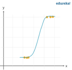
It is a classification algorithm in machine learning that uses one or more independent variables to determine an outcome. The outcome is measured with a dichotomous variable meaning it will have only two possible outcomes.

The goal of logistic regression is to find a best-fitting relationship between the dependent variable and a set of independent variables. It is better than other binary classification algorithms like nearest neighbor since it quantitatively explains the factors leading to classification.

Advantages and Disadvantages

Logistic regression is specifically meant for classification, it is useful in understanding how a set of independent variables affect the outcome of the dependent variable.

The main disadvantage of the logistic regression algorithm is that it only works when the predicted variable is binary, it assumes that the data is free of missing values and assumes that the predictors are independent of each other.

Use Cases

• Identifying risk factors for diseases

• Word classification

• Weather Prediction

• Voting Applications

Learn more about logistic regression with python here.

Naive Bayes Classifier

It is a classification algorithm based on Bayes’s theorem which gives an assumption of independence among predictors. In simple terms, a Naive Bayes classifier assumes that the presence of a particular feature in a class is unrelated to the presence of any other feature.

Even if the features depend on each other, all of these properties contribute to the probability independently. Naive Bayes model is easy to make and is particularly useful for comparatively large data sets. Even with a simplistic approach, Naive Bayes is known to outperform most of the classification methods in machine learning. Following is the Bayes theorem to implement the Naive Bayes Theorem.

Advantages and Disadvantages

The Naive Bayes classifier requires a small amount of training data to estimate the necessary parameters to get the results. They are extremely fast in nature compared to other classifiers.

The only disadvantage is that they are known to be a bad estimator.

Use Cases

• Disease Predictions

• Document Classification

• Spam Filters

• Sentiment Analysis

Know more about the Naive Bayes Classifier here.

Stochastic Gradient Descent

It is a very effective and simple approach to fit linear models. Stochastic Gradient Descent is particularly useful when the sample data is in a large number. It supports different loss functions and penalties for classification.

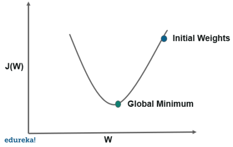
Stochastic gradient descent refers to calculating the derivative from each training data instance and calculating the update immediately.

Advantages and Disadvantages

The only advantage is the ease of implementation and efficiency whereas a major setback with stochastic gradient descent is that it requires a number of hyper-parameters and is sensitive to feature scaling.

Use Cases

• Internet Of Things

• Updating the parameters such as weights in neural networks or coefficients in linear regression

K-Nearest Neighbor

It is a lazy learning algorithm that stores all instances corresponding to training data in n-dimensional space. It is a lazy learning algorithm as it does not focus on constructing a general internal model, instead, it works on storing instances of training data.

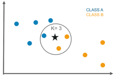
Classification is computed from a simple majority vote of the k nearest neighbors of each point. It is supervised and takes a bunch of labeled points and uses them to label other points. To label a new point, it looks at the labeled points closest to that new point also known as its nearest neighbors. It has those neighbors vote, so whichever label most of the neighbors have is the label for the new point. The “k” is the number of neighbors it checks.

Advantages And Disadvantages

This algorithm is quite simple in its implementation and is robust to noisy training data. Even if the training data is large, it is quite efficient. The only disadvantage with the KNN algorithm is that there is no need to determine the value of K and computation cost is pretty high compared to other algorithms.

Use Cases

• Industrial applications to look for similar tasks in comparison to others

• Handwriting detection applications

• Image recognition

• Video recognition

• Stock analysis

Know more about K Nearest Neighbor Algorithm here

Decision Tree

The decision tree algorithm builds the classification model in the form of a tree structure. It utilizes the if-then rules which are equally exhaustive and mutually exclusive in classification. The process goes on with breaking down the data into smaller structures and eventually associating it with an incremental decision tree. The final structure looks like a tree with nodes and leaves. The rules are learned sequentially using the training data one at a time. Each time a rule is learned, the tuples covering the rules are removed. The process continues on the training set until the termination point is met.

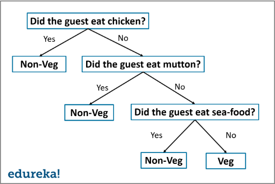
The tree is constructed in a top-down recursive divide and conquer approach. A decision node will have two or more branches and a leaf represents a classification or decision. The topmost node in the decision tree that corresponds to the best predictor is called the root node, and the best thing about a decision tree is that it can handle both categorical and numerical data.

Advantages and Disadvantages

A decision tree gives an advantage of simplicity to understand and visualize, it requires very little data preparation as well. The disadvantage that follows with the decision tree is that it can create complex trees that may bot categorize efficiently. They can be quite unstable because even a simplistic change in the data can hinder the whole structure of the decision tree.

Use Cases

• Data exploration

• Pattern Recognition

• Option pricing in finances

• Identifying disease and risk threats

Know more about decision tree algorithm here

Random Forest

Random decision trees or random forest are an ensemble learning method for classification, regression, etc. It operates by constructing a multitude of decision trees at training time and outputs the class that is the mode of the classes or classification or mean prediction(regression) of the individual trees.

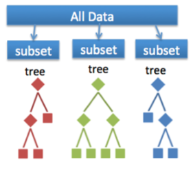
A random forest is a meta-estimator that fits a number of trees on various subsamples of data sets and then uses an average to improve the accuracy in the model’s predictive nature. The sub-sample size is always the same as that of the original input size but the samples are often drawn with replacements.

Advantages and Disadvantages

The advantage of the random forest is that it is more accurate than the decision trees due to the reduction in the over-fitting. The only disadvantage with the random forest classifiers is that it is quite complex in implementation and gets pretty slow in real-time prediction.

Use Cases

• Industrial applications such as finding if a loan applicant is high-risk or low-risk

• For Predicting the failure of  mechanical parts in automobile engines

• Predicting social media share scores

• Performance scores

Know more about the Random Forest algorithm here.

Artificial Neural Networks

A neural network consists of neurons that are arranged in layers, they take some input vector and convert it into an output. The process involves each neuron taking input and applying a function which is often a non-linear function to it and then passes the output to the next layer.

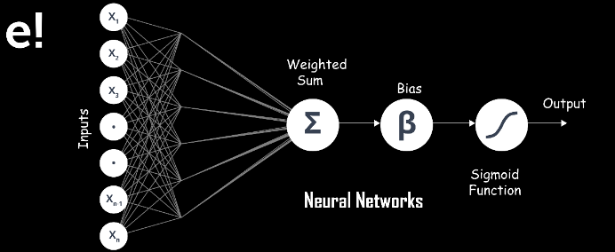
In general, the network is supposed to be feed-forward meaning that the unit or neuron feeds the output to the next layer but there is no involvement of any feedback to the previous layer.

Weighings are applied to the signals passing from one layer to the other, and these are the weighings that are tuned in the training phase to adapt a neural network for any problem statement.

Advantages and Disadvantages

It has a high tolerance to noisy data and able to classify untrained patterns, it performs better with continuous-valued inputs and outputs. The disadvantage with the artificial neural networks is that it has poor interpretation compared to other models.

Use Cases

• Handwriting analysis

• Colorization of black and white images

• Computer vision processes

• Captioning photos based on facial features

Know more about artificial neural networks here

Support Vector Machine

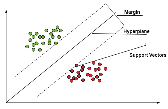
The support vector machine is a classifier that represents the training data as points in space separated into categories by a gap as wide as possible. New points are then added to space by predicting which category they fall into and which space they will belong to.

Advantages and Disadvantages

It uses a subset of training points in the decision function which makes it memory efficient and is highly effective in high dimensional spaces. The only disadvantage with the support vector machine is that the algorithm does not directly provide probability estimates.

Use cases

• Business applications for comparing the performance of a stock over a period of time

• Investment suggestions

• Classification of applications requiring accuracy and efficiency

Learn more about support vector machine in python here

Classifier Evaluation

The most important part after the completion of any classifier is the evaluation to check its accuracy and efficiency. There are a lot of ways in which we can evaluate a classifier. Let us take a look at these methods listed below.

Holdout Method

This is the most common method to evaluate a classifier. In this method, the given data set is divided into two parts as a test and train set 20% and 80% respectively.

The train set is used to train the data and the unseen test set is used to test its predictive power.

Cross-Validation

Over-fitting is the most common problem prevalent in most of the machine learning models. K-fold cross-validation can be conducted to verify if the model is over-fitted at all.

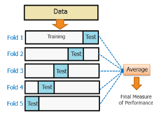
In this method, the data set is randomly partitioned into k mutually exclusive subsets, each of which is of the same size. Out of these, one is kept for testing and others are used to train the model. The same process takes place for all k folds.

Classification Report

A classification report will give the following results, it is a sample classification report of an SVM classifier using a cancer_data dataset.

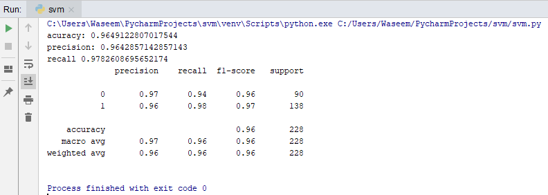
• Accuracy 

  • Accuracy is a ratio of correctly predicted observation to the total observations

  • True Positive: The number of correct predictions that the occurrence is positive.

  • True Negative: Number of correct predictions that the occurrence is negative.

• F1- Score

  • It is the weighted average of precision and recall

• Precision And Recall
  • Precision is the fraction of relevant instances among the retrieved instances, while recall is the fraction of relevant instances that have been retrieved over the total number of instances. They are basically used as the measure of relevance.

ROC Curve

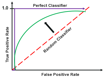
Receiver operating characteristics or ROC curve is used for visual comparison of classification models, which shows the relationship between the true positive rate and the false positive rate. The area under the ROC curve is the measure of the accuracy of the model.

Algorithm Selection

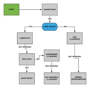
Apart from the above approach, We can follow the following steps to use the best algorithm for the model

• Read the data

• Create dependent and independent data sets based on our dependent and independent features

• Split the data into training and testing sets

• Train the model using different algorithms such as KNN, Decision tree, SVM, etc

• Evaluate the classifier

• Choose the classifier with the most accuracy.

Although it may take more time than needed to choose the best algorithm suited for your model, accuracy is the best way to go forward to make your model efficient.

Let us take a look at the MNIST data set, and we will use two different algorithms to check which one will suit the model best.

Use Case

What is MNIST?

It is a set of 70,000 small handwritten images labeled with the respective digit that they represent. Each image has almost 784 features, a feature simply represents the pixel’s density and each image is 28×28 pixels.

We will make a digit predictor using the MNIST dataset with the help of different classifiers.

Loading the MNIST dataset

from sklearn.datasets import fetch_openml
mnist = fetch_openml('mnist_784')
print(mnist)

Output:

Exploring The Dataset

import matplotlib
import matplotlib.pyplot as plt

X, y = mnist['data'], mnist['target']
random_digit = X[4800]
random_digit_image = random_digit.reshape(28,28)
plt.imshow(random_digit_image, cmap=matplotlib.cm.binary, interpolation="nearest")

Output: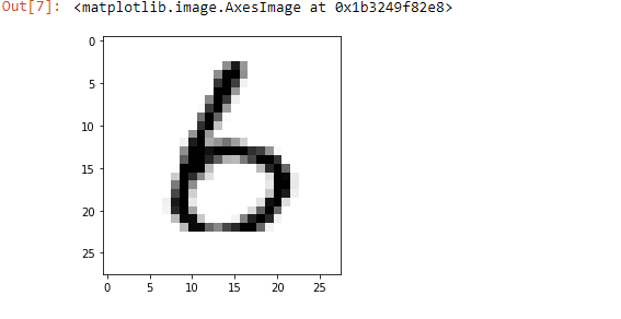

Splitting the Data

We are using the first 6000 entries as the training data, the dataset is as large as 70000 entries. You can check using the shape of the X and y. So to make our model memory efficient, we have only taken 6000 entries as the training set and 1000 entries as a test set.

x_train, x_test = X[:6000], X[6000:7000]
y_train, y_test = y[:6000], y[6000:7000]

Shuffling The Data

To avoid unwanted errors, we have shuffled the data using the numpy array. It basically improves the efficiency of the model.

import numpy as np

shuffle_index = np.random.permutation(6000)
x_train, y_train = x_train[shuffle_index], y_train[shuffle_index]

Creating A Digit Predictor Using Logistic Regression

y_train = y_train.astype(np.int8)
y_test = y_test.astype(np.int8)
y_train_2 = (y_train==2)
y_test_2 = (y_test==2)
print(y_test_2)

Output : 

from sklearn.linear_model import LogisticRegression
clf = LogisticRegression(tol=0.1)
clf.fit(x_train,y_train_2)
clf.predict([random_digit])

Output:

Cross-Validation 

from sklearn.model_selection import cross_val_score 
a = cross_val_score(clf, x_train, y_train_2, cv=3, scoring="accuracy")
a.mean()

Output:

Creating A Predictor Using Support Vector Machine

from sklearn import svm

cls = svm.SVC()
cls.fit(x_train, y_train_2)
cls.predict([random_digit])

Output:

Cross-Validation

a = cross_val_score(cls, x_train, y_train_2, cv = 3, scoring="accuracy")
a.mean()

Output:

In the above example, we were able to make a digit predictor. Since we were predicting if the digit were 2 out of all the entries in the data, we got false in both the classifiers, but the cross-validation shows much better accuracy with the logistic regression classifier instead of the support vector machine classifier.

This brings us to the end of this article where we have learned Classification in Machine Learning. I hope you are clear with all that has been shared with you in this tutorial.

You can also take a Machine Learning Course Masters Program. The program will provide you with the most in-depth and practical information on machine-learning applications in real-world situations. Additionally, you’ll learn the essentials needed to be successful in the field of machine learning, such as statistical analysis, Python, and data science.

Also, if you’re looking to develop the career you’re in with Deep learning, you should take a look at the Deep Learning Course. This course gives students information about the techniques, tools, and techniques they need to grow their careers.

We are here to help you with every step on your journey and come up with a curriculum that is designed for students and professionals who want to be a Python developer. The course is designed to give you a head start into Python programming and train you for both core and advanced Python concepts along with various Python frameworks like Django.

If you come across any questions, feel free to ask all your questions in the comments section of “Classification In Machine Learning” and our team will be glad to answer.