Introduction to Classification Algorithms

The idea of Classification Algorithms is pretty simple. You predict the target class by analyzing the training dataset. This is one of the most, if not the most essential concept you study when you learn Data Science.

This blog discusses the following concepts:

• What is Classification?
• Classification vs Clustering Algorithms
• Basic Terminology in Classification Algorithm
• Applications of Classification Algorithm
• Types of Classification Algorithm
• Logistic Regression
• Decision Tree
• Naive Bayes Classifier
• K Nearest Neighbour
• SVM 

What is Classification? 

We use the training dataset to get better boundary conditions which could be used to determine each target class. Once the boundary conditions are determined, the next task is to predict the target class. The whole process is known as classification.

Target class examples:

• Analysis of the customer data to predict whether he will buy computer accessories (Target class: Yes or No)
• Classifying fruits from features like color, taste, size, weight (Target classes: Apple, Orange, Cherry, Banana)
• Gender classification from hair length (Target classes: Male or Female)

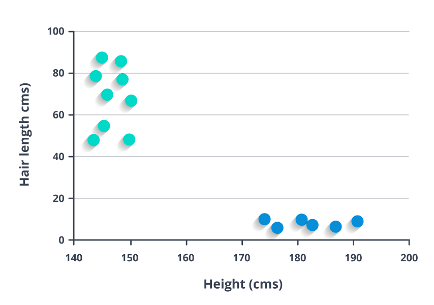
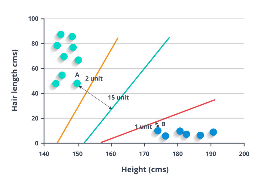
Let’s understand the concept of classification algorithms with gender classification using hair length (by no means am I trying to stereotype by gender, this is only an example). To classify gender (target class) using hair length as feature parameter we could train a model using any classification algorithms to come up with some set of boundary conditions which can be used to differentiate the male and female genders using hair length as the training feature. In gender classification case the boundary condition could the proper hair length value. Suppose the differentiated boundary hair length value is 15.0 cm then we can say that if hair length is less than 15.0 cm then gender could be male or else female.

Classification Algorithms vs Clustering Algorithms

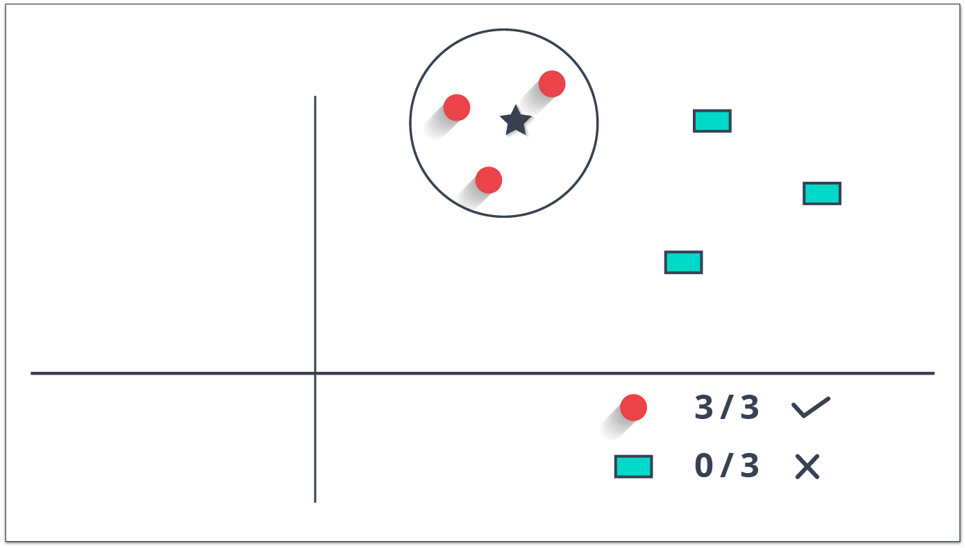
In clustering, the idea is not to predict the target class as in classification, it’s more ever trying to group the similar kind of things by considering the most satisfied condition, all the items in the same group should be similar and no two different group items should not be similar.  

Group items Examples:

• While grouping similar language type documents (Same language documents are one group.)
• While categorizing the news articles (Same news category(Sport) articles are one group )

Let’s understand the concept with clustering genders based on hair length example. To determine gender, different similarity measure could be used to categorize male and female genders. This could be done by finding the similarity between two hair lengths and keep them in the same group if the similarity is less (Difference of hair length is less). The same process could continue until all the hair length properly grouped into two categories.

Basic Terminology in Classification Algorithms

• Classifier: An algorithm that maps the input data to a specific category.
• Classification model: A classification model tries to draw some conclusion from the input values given for training. It will predict the class labels/categories for the new data.
• Feature: A feature is an individual measurable property of a phenomenon being observed.
• Binary Classification: Classification task with two possible outcomes. Eg: Gender classification (Male / Female)
• Multi-class classification: Classification with more than two classes. In multi-class classification, each sample is assigned to one and only one target label. Eg: An animal can be a cat or dog but not both at the same time. 
• Multi-label classification: Classification task where each sample is mapped to a set of target labels (more than one class). Eg: A news article can be about sports, a person, and location at the same time.

Applications of Classification Algorithms

• Email spam classification
• Bank customers loan pay willingness prediction.
• Cancer tumor cells identification.
• Sentiment analysis 
• Drugs classification
• Facial key points detection
• Pedestrians detection in an automotive car driving.

Types of Classification Algorithms

Classification Algorithms could be broadly classified as the following:

• Linear Classifiers
  • Logistic regression
  • Naive Bayes classifier
  • Fisher’s linear discriminant
• Support vector machines
  • Least squares support vector machines
• Quadratic classifiers
• Kernel estimation
  • k-nearest neighbor 
• Decision trees
  • Random forests
• Neural networks
• Learning vector quantization

Examples of a few popular Classification Algorithms are given below.

Logistic Regression

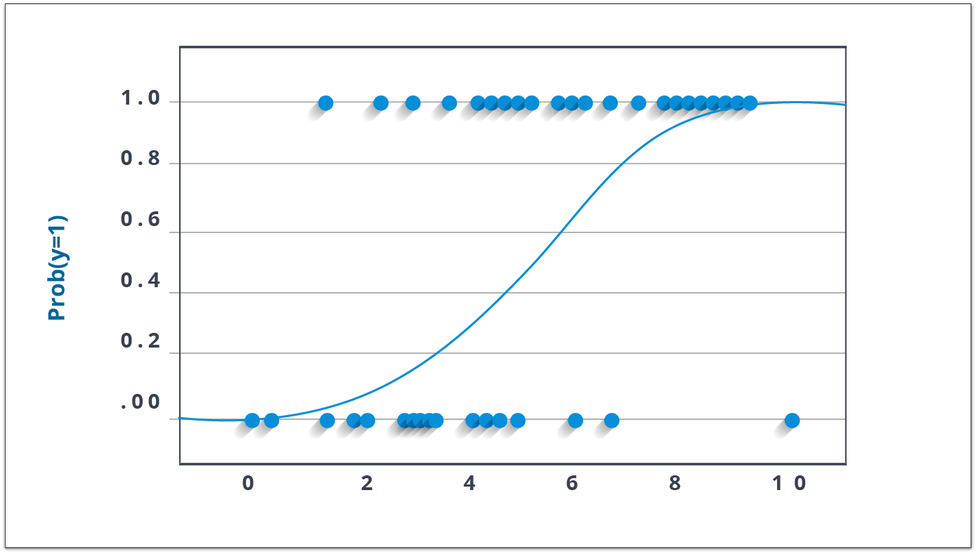
As confusing as the name might be, you can rest assured. Logistic Regression is a classification and not a regression algorithm. It estimates discrete values (Binary values like 0/1, yes/no, true/false) based on a given set of independent variable(s). Simply put, it basically, predicts the probability of occurrence of an event by fitting data to a logit function. Hence, it is also known as logit regression. The values obtained would always lie within 0 and 1 since it predicts the probability.

Let us try and understand this through another example.

Let’s say there’s a sum on your math test. It can only have 2 outcomes, right? Either you solve it or you don’t (and let’s not assume points for method here). Now imagine, that you are being given a wide range of sums in an attempt to understand which chapters have you understood well. The outcome of this study would be something like this – if you are given a trigonometry based problem, you are 70% likely to solve it. On the other hand, if it is an arithmetic problem, the probability of you getting an answer is only 30%. This is what Logistic Regression provides you.

If I had to do the math, I would model the log odds of the outcome as a linear combination of the predictor variables.

odds= p/ (1-p) = probability of event occurrence / probability of event occurrence ln(odds) = ln(p/(1-p)) logit(p) = ln(p/(1-p)) = b0+b1X1+b2X2+b3X3....+bkXk)

In the equation given above, p is the probability of the presence of the characteristic of interest. It chooses parameters that maximize the likelihood of observing the sample values rather than that minimize the sum of squared errors (like in ordinary regression).

Now, a lot of you might wonder, why take a log? For the sake of simplicity, let’s just say that this is one of the best mathematical ways to replicate a step function. I can go way more in-depth with this, but that will beat the purpose of this blog.

R-Code:

x <- cbind(x_train,y_train)
# Train the model using the training sets and check score
logistic <- glm(y_train ~ ., data = x,family='binomial')
summary(logistic)
#Predict Output
predicted= predict(logistic,x_test)

There are many different steps that could be tried in order to improve the model: 

• include interaction terms
• remove features
• regularize techniques
• use a non-linear model

Decision Trees

Now, the decision tree is by far, one of my favorite algorithms. With versatile features helping actualize both categorical and continuous dependent variables, it is a type of supervised learning algorithm mostly used for classification problems. What this algorithm does is, it splits the population into two or more homogeneous sets based on the most significant attributes making the groups as distinct as possible.

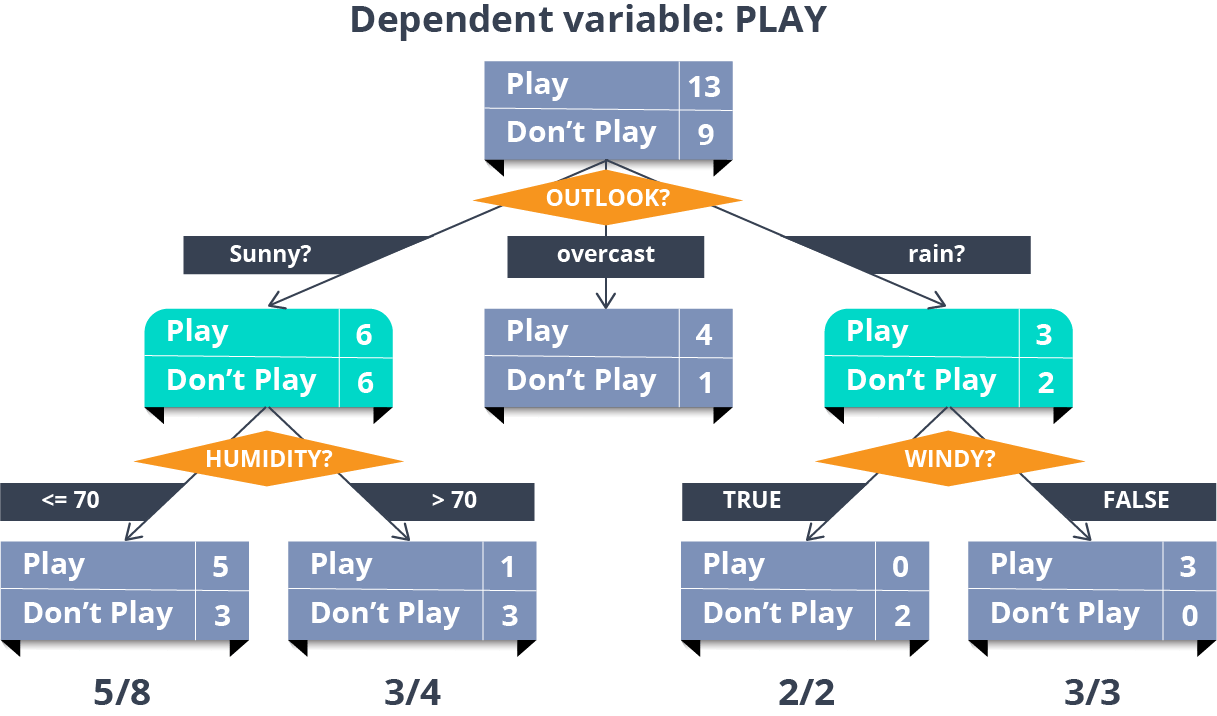
In the image above, you can see that population is classified into four different groups based on multiple attributes to identify ‘if they will play or not’. 

R-Code:

library(rpart)
x <- cbind(x_train,y_train)
# grow tree 
fit <- rpart(y_train ~ ., data = x,method="class")
summary(fit)
#Predict Output 
predicted= predict(fit,x_test)

Naive Bayes Classifier

This is a classification technique based on an assumption of independence between predictors or what’s known as Bayes’ theorem. In simple terms, a Naive Bayes classifier assumes that the presence of a particular feature in a class is unrelated to the presence of any other feature.

For example, a fruit may be considered to be an apple if it is red, round, and about 3 inches in diameter. Even if these features depend on each other or upon the existence of the other features, a Naive Bayes Classifier would consider all of these properties to independently contribute to the probability that this fruit is an apple.

To build a Bayesian model is simple and particularly functional in case of enormous data sets. Along with simplicity, Naive Bayes is known to outperform sophisticated classification methods as well.

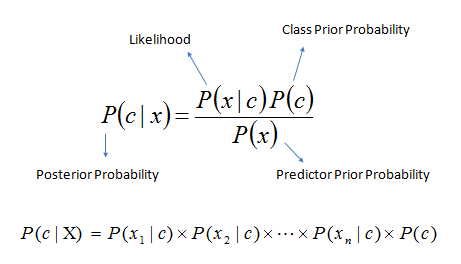
Bayes theorem provides a way of calculating posterior probability P(c|x) from P(c), P(x) and P(x|c). The expression for Posterior Probability is as follows.

Here,

• P(c|x) is the posterior probability of class (target) given predictor (attribute). 
• P(c) is the prior probability of class. 
• P(x|c) is the likelihood which is the probability of predictor given class. 
• P(x) is the prior probability of predictor.

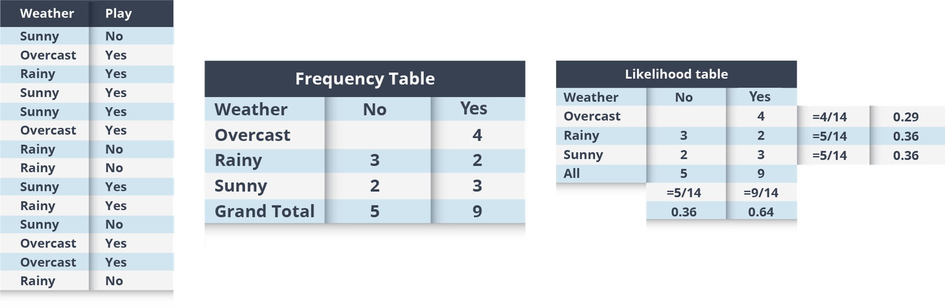
Example: Let’s work through an example to understand this better. So, here I have a training data set of weather namely, sunny, overcast and rainy, and corresponding binary variable ‘Play’. Now, we need to classify whether players will play or not based on weather condition. Let’s follow the below steps to perform it.

Step 1: Convert the data set to the frequency table

Step 2: Create a Likelihood table by finding the probabilities like Overcast probability = 0.29 and probability of playing is 0.64.

Step 3: Now, use the Naive Bayesian equation to calculate the posterior probability for each class. The class with the highest posterior probability is the outcome of prediction.

Problem: Players will play if the weather is sunny, is this statement correct?

We can solve it using above discussed method, so P(Yes | Sunny) = P( Sunny | Yes) * P(Yes) / P (Sunny)

Here we have P (Sunny |Yes) = 3/9 = 0.33, P(Sunny) = 5/14 = 0.36, P( Yes)= 9/14 = 0.64

Now, P (Yes | Sunny) = 0.33 * 0.64 / 0.36 = 0.60, which has higher probability.

Naive Bayes uses a similar method to predict the probability of different class based on various attributes. This algorithm is mostly used in text classification and with problems having multiple classes. 

R-Code:

library(e1071)
x <- cbind(x_train,y_train)
# Fitting model
fit <-naiveBayes(y_train ~ ., data = x)
summary(fit)
#Predict Output 
predicted= predict(fit,x_test)

KNN (k- Nearest Neighbors)

K nearest neighbors is a simple algorithm used for both classification and regression problems. It basically stores all available cases to classify the new cases by a majority vote of its k neighbors. The case assigned to the class is most common amongst its K nearest neighbors measured by a distance function (Euclidean, Manhattan, Minkowski, and Hamming).

While the three former distance functions are used for continuous variables, Hamming distance function is used for categorical variables. If K = 1, then the case is simply assigned to the class of its nearest neighbor. At times, choosing K turns out to be a challenge while performing kNN modeling.

You can understand KNN easily by taking an example of our real lives. If you have a crush on a girl/boy in class, of whom you have no information, you might want to talk to their friends and social circles to gain access to their information!

R-Code:

library(knn)
x <- cbind(x_train,y_train)
# Fitting model
fit <-knn(y_train ~ ., data = x,k=5)
summary(fit)
#Predict Output 
predicted= predict(fit,x_test)

Things to consider before selecting KNN: 

• KNN is computationally expensive
• Variables should be normalized else higher range variables can bias it
• Works on pre-processing stage more before going for kNN like an outlier, noise removal

SVM(Support Vector Machine)

In this algorithm, we plot each data item as a point in n-dimensional space (where n is a number of features you have) with the value of each feature being the value of a particular coordinate.

For example, if we only had two features like Height and Hair length of an individual, we’d first plot these two variables in two-dimensional space where each point has two coordinates (these coordinates are known as Support Vectors)

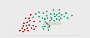
Now, we will find some line that splits the data between the two differently classified groups of data. This will be the line such that the distances from the closest point in each of the two groups will be farthest away.

In the example shown above, the line which splits the data into two differently classified groups is the blue line, since the two closest points are the farthest apart from the line. This line is our classifier. Then, depending on where the testing data lands on either side of the line, that’s what class we can classify the new data as.

R-Code:

library(e1071)
x <- cbind(x_train,y_train)
# Fitting model
fit <-svm(y_train ~ ., data = x)
summary(fit)
#Predict Output 
predicted= predict(fit,x_test)

So, with this, we come to the end of this Classification Algorithms Blog. Try out the simple R-Codes on your systems now and you’ll no longer call yourselves newbies in this concept.