


Advanced Power BI Certification Course with G ...
- 13k Enrolled Learners
- Weekend
- Live Class
(4230)


 Copy Link!
Data comes to use only when you can actually work on it and Excel is one tool that provides a great amount of convenience both when you have to formulate equations of your own or make use of the built-in ones. In this article, you will be learning how you can actually work with these Excel Formulas ad Functions.
Here is a quick look at the topics that are discussed over here:
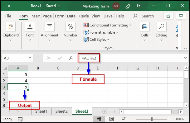
In general, a formula is a condensed way of representing some information in terms of symbols. In Excel, formulas are expressions that can be entered into the cells of an Excel sheet and their outputs are displayed as a result.
Excel formulas can be of the following types:
Type | Example | Description |
Mathematical operators( +, -, *, etc) | Example: =A1+B1 | Adds the values of A1 and B1 |
Values or text | Example: 100*0.5 multiples 100 times 0.5 | Takes the values and returns the output |
Cell reference | EXAMPLE: =A1=B1 | Returns TRUE or FALSE by comparing A1 and B1 |
Worksheet functions | EXAMPLE: =SUM(A1: B1) | Returns the output by adding values present in A1 and B1 |
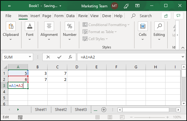
In order to write a formula to an Excel sheet cell, you can do as follows:
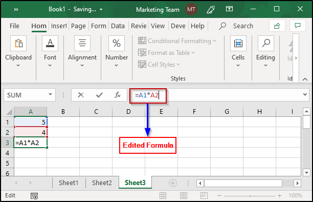
In case you want to edit some previously entered formula, simply select the cell that contains the target formula and in the formula bar you can make the desired changes. In the previous example, I have calculated the Sum of A1 and A2. Now, I will edit the same and change the formula to calculate the product of the values present in these two cells:
Once this is done, press Enter to see the desired output.
Excel comes in really handy when you have to copy/ paste formulas. Whenever you copy a formula, Excel automatically takes care of the cell references that are required at that position. This is done through a system called as Relative Cell Addresses.
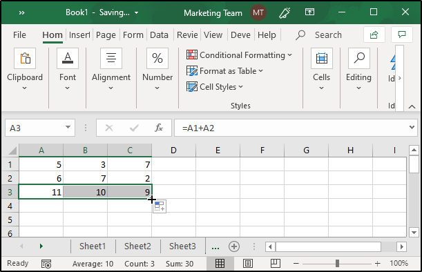
To copy a formula, select the cell that holds the original formula and then drag it till that cell which requires a copy of that formula as follows:
As you can see in the image, the formula is written originally in A3 and then I have dragged it down along B3 and C3 to calculate the sum of B1, B2 and C1, C2 without exclusively writing down the cell addresses.
In case I change the values of any of the cells, the output will be updated automatically by Excel in accordance with the Relative Cell Addresses, Absolute Cell Addresses or Mixed Cell Addresses.
In case you want to hide some formula from an excel sheet, you can do it as follows:
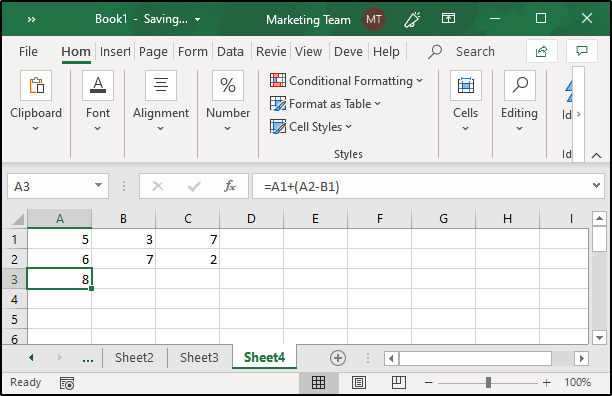
Excel formulas follow the BODMAS (Brackets Order Division Multiplication Addition Subtraction) rules. If you have a formula that contains brackets, the expression within the brackets will be solved before any other part of the complete formula. Take a look at the image below:
As you can see in the above example, I have a formula that consists of a bracket. So in accordance with the BODMAS rules, Excel will first find the difference between A2 and B1 and then it adds the result with A1.
In general, a function defines a formula that is executed in some given order. Excel provides a huge number of built-in functions that can be used in order to calculate the result of various formulas.
Formulas in Excel are divided into the following categories:
Now, let us check out how to make use of some of the most important and commonly used Excel Formulas.
Here are some of the most important Excel functions along with their descriptions and examples.
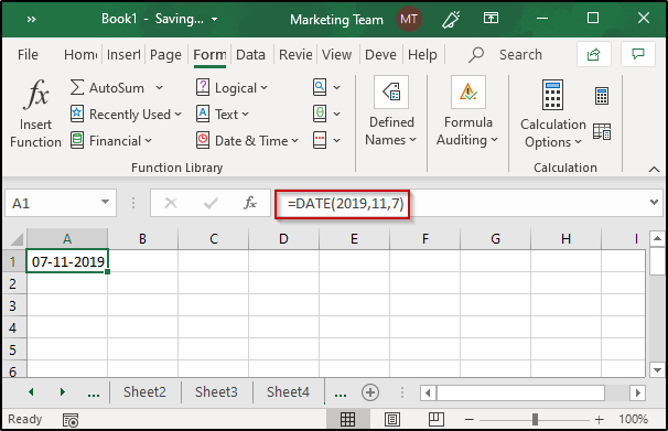
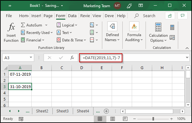
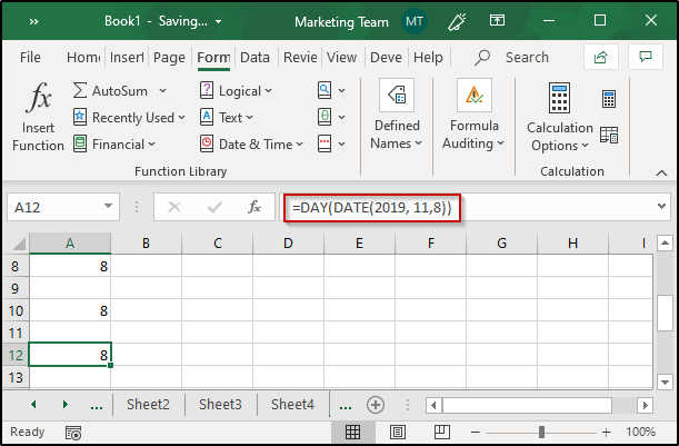
One of the most important and widely used Date function in Excel is the DATE function. The syntax of it is as follows:
DATE(year, month, day)
This function returns a number that represents the given date in the MS Excel date-time format. The DATE function can be used as follows:
EXAMPLE:
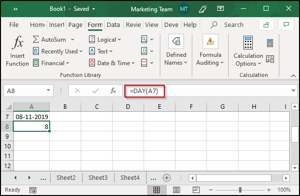
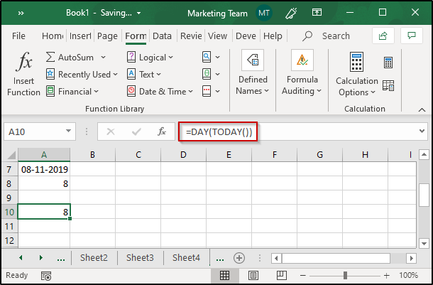
This function returns the day value of the month (1-31). The syntax of it is as follows:
DAY(serial_number)
Here, serial_number is the date whose day you want to retrieve. It can be given in any manner such as the result of some other function, supplied by the DATE function, or a cell reference.
EXAMPLE:
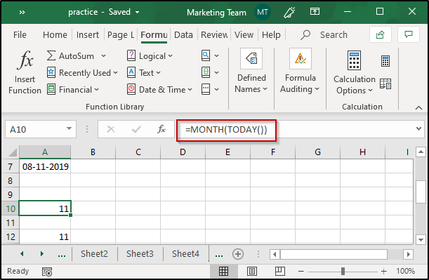
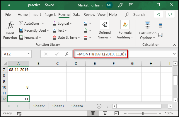
Just like the DAY function, Excel provides another function i.e the MONTH function to retrieve the month from a specific date. The syntax is as follows:
MONTH(serial_number)
EXAMPLE:
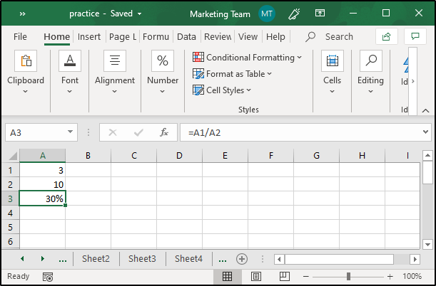
As we all know, Percentage is the ratio calculated as a fraction of 100. It can be denoted as follows:
Percentage = (Part/ Whole) x 100
In Excel, you can calculate the percentage of any desired values. For example, if you have the part and whole values present in A1 and A2 and you want to calculate the percentage, you can do it as follows:
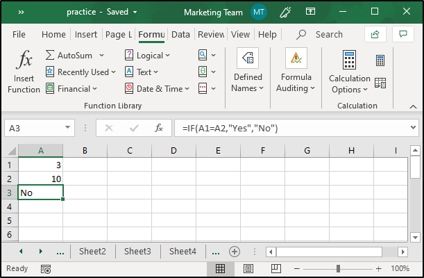
The IF statement is a conditional statement that returns True when the specified condition is satisfied and Flase when the condition is not. Excel provides a built-in “IF” function that serves this purpose. Its syntax is as follows:
IF(logical_test, value_if_true, value_if_false)
Here, logical_test is the condition that is to be checked
EXAMPLE:
This function is used in order to look up and fetch some particular data from a column from an Excel sheet. The “V” in VLOOKUP stands for vertical lookup. It is one of the most important and widely used formulas in Excel and in order to use this function, the table must be sorted in ascending order. The syntax of this function is as follows:
VLOOKUP(lookup_value, table_array, col_index, num_range, lookup)
where,
lookup_value is the value to be searched
table_array is the table that is to be searched
col_index is the column from which the value is to be retrieved
range_lookup (optional) returns TRUE for approx. match and FALSE for an exact match
EXAMPLE:
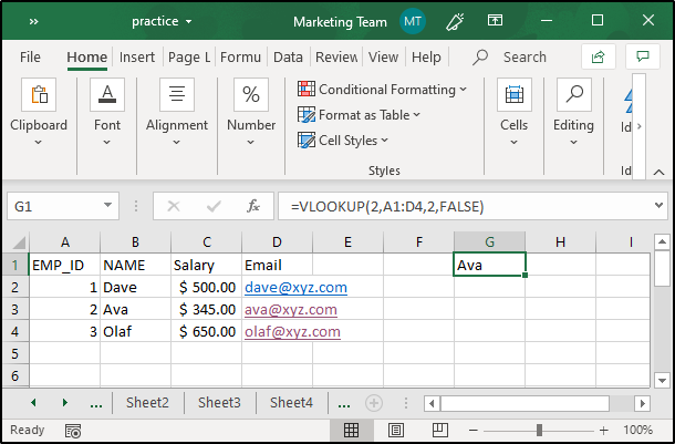
As you can see in the image, the value that I have specified is 2 and the table range is between A1 and D4. I want to fetch the name of the employee, therefore I have given the column value as 2 and since I want it to be an exact match, I used False for range lookup.
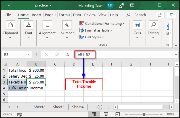
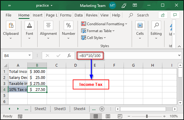
Suppose you want to calculate the income tax of a person whose total salary is $300. You will need to calculate the income tax as follows:
The SUM function in Excel calculates the result by adding all the specified values in Excel. The syntax of this function is as follows:
SUM(number1, number2, …)
Adds all the numbers that are specified as a parameter to it.
EXAMPLE:
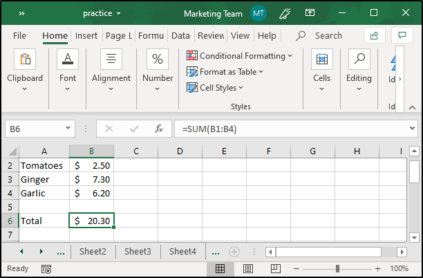
In case you want to calculate the sum of the amount you spent in purchasing vegetables, list down all the prices and then use the SUM formula as follows:
To calculate compound interest, you can make use of one of the Excel Formulas called FV. This function will return the future value of an investment on the basis of periodic, constant interest rate and payments. The syntax of this function is as follows:
FV(rate, nper, pmt, pv, type)
In order to calculate the rate, you will need to divide the annual rate by the number of periods i.e annual rate/ periods. No. of periods or nper is calculated by multiplying the term (no. of years) with the periods i.e term * periods. pmt stands for periodic payment and can be any value including zero.
Consider the following example:
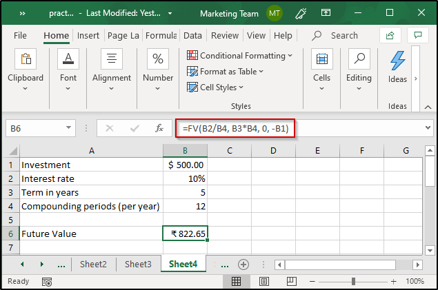
In the above example, I have calculated the Compound Interest for $500 at a rate of 10% for 5 years and assuming that the periodic payment value is 0. Please note that I have used -B1 meaning, $500 has been taken from me.
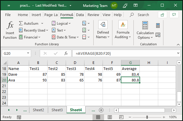
The average, as we all know, depicts the median value of a number of values. In Excel, the average can be easily calculated using the built-in function called “AVERAGE”. The syntax of this function is as follows:
AVERAGE(number1, number2, …)
EXAMPLE:
In case you want to calculate the average marks attained by students in all the exams, you can simply create a table and then use the AVERAGE formula to calculate the average marks attained by each student.
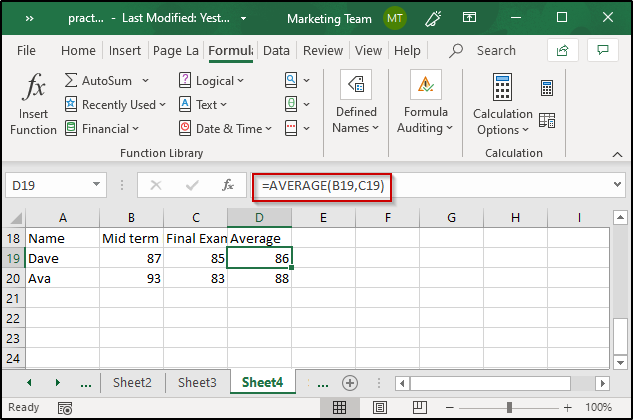
In the above example, I have calculated the average marks for two students in two exams. In case you have more than two values whose average needs to be determined, you just have to specify the range of cells wherein the values are present. For example:
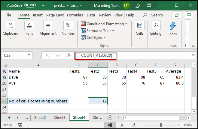
The count function in Excel will count the number of cells containing numbers in a given range. The syntax of this function is as follows:
COUNT(value1, value2, …)
EXAMPLE:
In case I want to calculate the number of cells holding numbers from the table I created in the previous example, I will simply have to select the cell wherein I want to display the result and then make use of the COUNT function as follows:
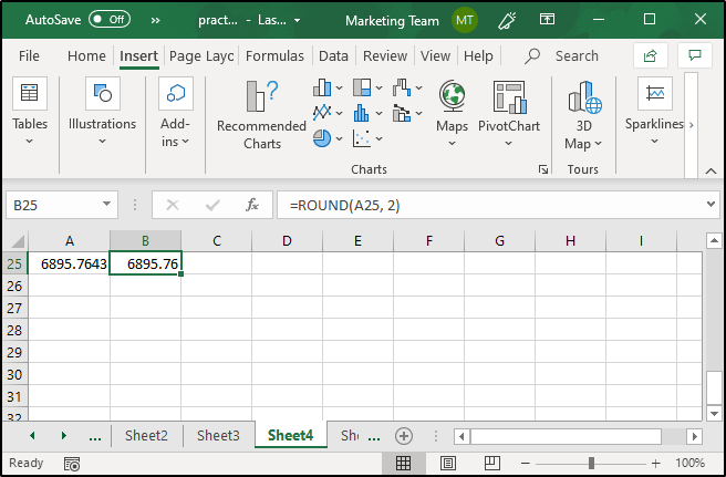
In order to round off values to some specific decimal places, you can make use of the ROUND function. This function will return a number by rounding it off to the specified number of decimal places. The syntax of this function is as follows:
ROUND(number, num_digits)
EXAMPLE:
In order to find grades, you will have to make use of nested IF statements in Excel. For example, in the Average example, I had calculated the average marks scored by students in the tests. Now, to find the Grades attained by these students, I will have to create a nested IF function as follows:

As you can see, the average marks are present in column G. To calculate the grade, I have used a nested IF formula. The code is as follows:
=IF(G19>90,”A”,(IF(G19>75,”B”,IF(G19>60,”C”,IF(G19>40,”D”,”F”)))))
After doing this, you will just have to copy the formula to all the cells where you want to display the grades.
In case you want to determine the Rank attained by the students of a class, you can make use of one of the built-in Excel Formulas i.e RANK. This function will return the Rank for a specified range by comparing a given range in the ascending or in the descending order. The syntax of this function is as follows:
RANK(ref, number, order)
EXAMPLE:
![]()
As you can see, in the above example, I have calculated the Rank of the students using the Rank function. Here, the first parameter is the average marks attained by each student and the array is the average attained by all other students of the class. I have not specified any order, therefore, the output will be determined in the descending order. For ascending order ranks, you will have to specify any nonzero value.
In order to count the cells based on some given condition, you can use one of the built-in Excel Formulas called “COUNTIF”. This function will return the number of cells that satisfy some condition in a given range. The syntax of this function is as follows:
COUNTIF(range, criteria)
EXAMPLE:
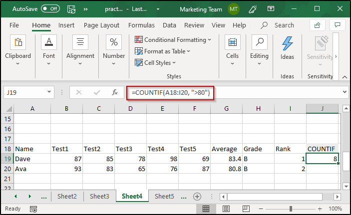
As you can see, in the above example, I have found the number of cells having values that are greater than 80. You can also give some text value to the criteria parameter.
The INDEX function returns a value or cell reference at some particular position in a specified range. The syntax of this function is as follows:
INDEX(array, row_num, column_num) or
INDEX(reference, row_num, column_num, area_num)
The index function works as follows for the Array form:
The index function works as follows for the Reference form:
EXAMPLE:
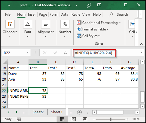
As you can see, in the above example, I have used the INDEX function to determine the value present in the 2nd row and 4th column for the range of cells between A18 to G20.
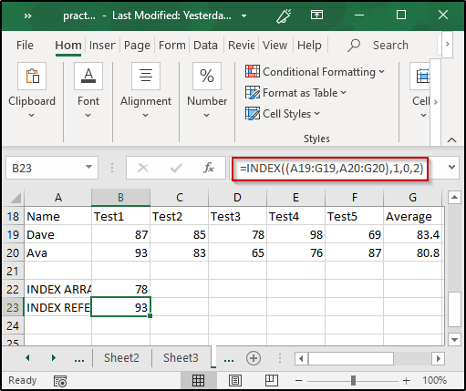
Similarly, you can also use the INDEX function by specifying multiple references as follows:
This brings us to the end of this article on Excel Formulas and Functions. I hope you are clear with all that has been shared with you. Make sure you practice as much as possible and revert your experience. Supercharge your Excel skills with our complete guide to formulas and functions, and Excel Interview questions for your next interview with confidence!
To get in-depth knowledge on any trending technologies along with its various applications, you can enroll for live Edureka MS Excel Online training with 24/7 support and lifetime access. Also, Don’t miss out on this opportunity to enhance your career prospects and become a sought-after business intelligence professional. Click the link below to enroll in our MSBI Course now!
Got a question for us? Please mention it in the comments section of this “Excel Formulas and Functions” blog and we will get back to you as soon as possible.


 Thank you for registering Join Edureka Meetup community for 100+ Free Webinars each month JOIN MEETUP GROUP