


Artificial Intelligence encircles a wide range of technologies and techniques that enable computer systems to solve problems like Data Compression which is used in computer vision, computer networks, computer architecture, and many other fields. Autoencoders are unsupervised neural networks that use machine learning to do this compression for us. This Autoencoders Tutorial will provide you with a complete insight into autoencoders in the following sequence:
- What are Autoencoders?
- The need for Autoencoders
- Applications of Autoencoders
- Architecture of Autoencoders
- Properties & Hyperparameters
- Types of Autoencoders
- Data Compression using Autoencoders (Demo)
Let’s begin with the most fundamental and essential question, What are autoencoders?
What are Autoencoders?
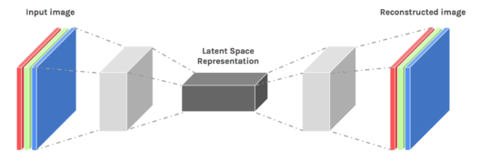
An autoencoder neural network is an Unsupervised Machine learning algorithm that applies backpropagation, setting the target values to be equal to the inputs. Autoencoders are used to reduce the size of our inputs into a smaller representation. If anyone needs the original data, they can reconstruct it from the compressed data.

We have a similar machine learning algorithm ie. PCA which does the same task. So you might be thinking why do we need Autoencoders then? Let’s continue this Autoencoders Tutorial and find out the reason behind using Autoencoders.
Autoencoders Tutorial: Its Emergence
Autoencoders are preferred over PCA because:
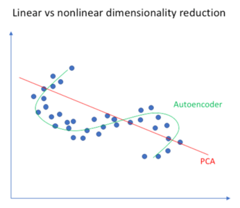

- An autoencoder can learn non-linear transformations with a non-linear activation function and multiple layers.
- It doesn’t have to learn dense layers. It can use convolutional layers to learn which is better for video, image and series data.
- It is more efficient to learn several layers with an autoencoder rather than learn one huge transformation with PCA.
- An autoencoder provides a representation of each layer as the output.
- It can make use of pre-trained layers from another model to apply transfer learning to enhance the encoder/decoder.
Now let’s have a look at a few Industrial Applications of Autoencoders.
Subscribe to our youtube channel to get new updates..!
Applications of Autoencoders
Image Coloring


Autoencoders are used for converting any black and white picture into a colored image. Depending on what is in the picture, it is possible to tell what the color should be.

Feature variation
It extracts only the required features of an image and generates the output by removing any noise or unnecessary interruption.

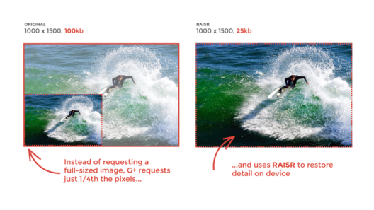
Dimensionality Reduction
The reconstructed image is the same as our input but with reduced dimensions. It helps in providing the similar image with a reduced pixel value.

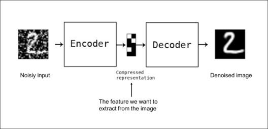
Denoising Image
The input seen by the autoencoder is not the raw input but a stochastically corrupted version. A denoising autoencoder is thus trained to reconstruct the original input from the noisy version.


Watermark Removal
It is also used for removing watermarks from images or to remove any object while filming a video or a movie.
Now that you have an idea of the different industrial applications of Autoencoders, let’s continue our Autoencoders Tutorial Blog and understand the complex architecture of Autoencoders.
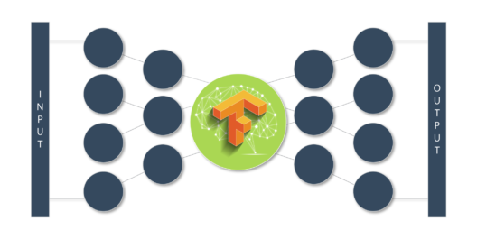
Architecture of Autoencoders
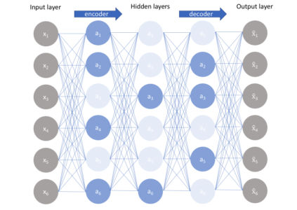
An Autoencoder consist of three layers:
- Encoder
- Code
- Decoder
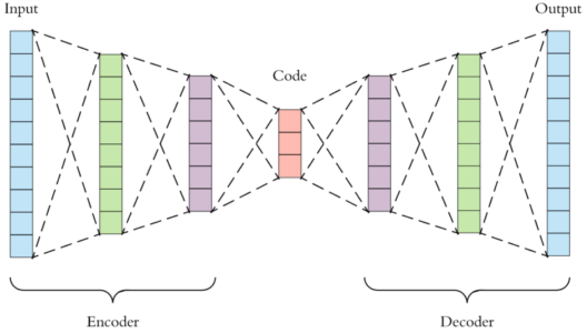

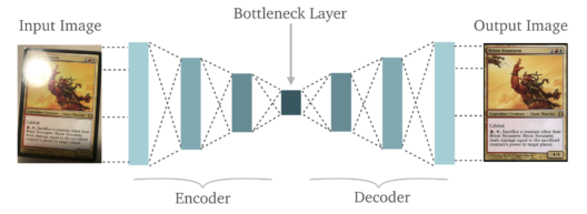
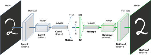
- Encoder: This part of the network compresses the input into a latent space representation. The encoder layer encodes the input image as a compressed representation in a reduced dimension. The compressed image is the distorted version of the original image.
- Code: This part of the network represents the compressed input which is fed to the decoder.
- Decoder: This layer decodes the encoded image back to the original dimension. The decoded image is a lossy reconstruction of the original image and it is reconstructed from the latent space representation.
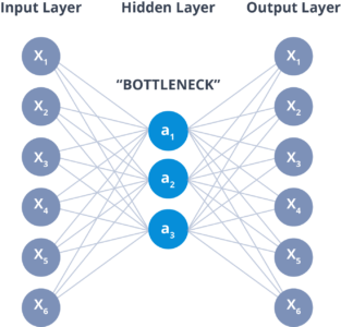

The layer between the encoder and decoder, ie. the code is also known as Bottleneck. This is a well-designed approach to decide which aspects of observed data are relevant information and what aspects can be discarded. It does this by balancing two criteria :
- Compactness of representation, measured as the compressibility.
- It retains some behaviourally relevant variables from the input.
Now that you have an idea of the architecture of an Autoencoder. Let’s continue our Autoencoders Tutorial and understand the different properties and the Hyperparameters involved while training Autoencoders.
Properties and Hyperparameters
Properties of Autoencoders:
- Data-specific: Autoencoders are only able to compress data similar to what they have been trained on.
- Lossy: The decompressed outputs will be degraded compared to the original inputs.
- Learned automatically from examples: It is easy to train specialized instances of the algorithm that will perform well on a specific type of input.
Hyperparameters of Autoencoders:
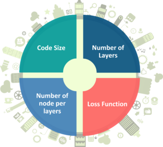

There are 4 hyperparameters that we need to set before training an autoencoder:
- Code size: It represents the number of nodes in the middle layer. Smaller size results in more compression.
- Number of layers: The autoencoder can consist of as many layers as we want.
- Number of nodes per layer: The number of nodes per layer decreases with each subsequent layer of the encoder, and increases back in the decoder. The decoder is symmetric to the encoder in terms of the layer structure.
- Loss function: We either use mean squared error or binary cross-entropy. If the input values are in the range [0, 1] then we typically use cross-entropy, otherwise, we use the mean squared error.
Now that you know the properties and hyperparameters involved in the training of Autoencoders. Let’s move forward with our Autoencoders Tutorial and understand the different types of autoencoders and how they differ from each other.
Types of Autoencoders
Convolution Autoencoders
Autoencoders in their traditional formulation does not take into account the fact that a signal can be seen as a sum of other signals. Convolutional Autoencoders use the convolution operator to exploit this observation. They learn to encode the input in a set of simple signals and then try to reconstruct the input from them, modify the geometry or the reflectance of the image.

Use cases of CAE:
- Image Reconstruction
- Image Colorization
- latent space clustering
- generating higher resolution images
Sparse Autoencoders
Sparse autoencoders offer us an alternative method for introducing an information bottleneck without requiring a reduction in the number of nodes at our hidden layers. Instead, we’ll construct our loss function such that we penalize activations within a layer.

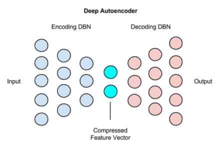
Deep Autoencoders
The extension of the simple Autoencoder is the Deep Autoencoder. The first layer of the Deep Autoencoder is used for first-order features in the raw input. The second layer is used for second-order features corresponding to patterns in the appearance of first-order features. Deeper layers of the Deep Autoencoder tend to learn even higher-order features.
A deep autoencoder is composed of two, symmetrical deep-belief networks-
- First four or five shallow layers representing the encoding half of the net.
- The second set of four or five layers that make up the decoding half.

Use cases of Deep Autoencoders
- Image Search
- Data Compression
- Topic Modeling & Information Retrieval (IR)
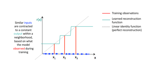
Contractive Autoencoders
A contractive autoencoder is an unsupervised deep learning technique that helps a neural network encode unlabeled training data. This is accomplished by constructing a loss term which penalizes large derivatives of our hidden layer activations with respect to the input training examples, essentially penalizing instances where a small change in the input leads to a large change in the encoding space.

Now that you have an idea of what Autoencoders is, it’s different types and it’s properties. Let’s move ahead with our Autoencoders Tutorial and understand a simple implementation of it using TensorFlow in Python.
Subscribe to our youtube channel to get new updates..!
Data Compression using Autoencoders(Demo)

Let’s import the required libraries
import numpy as np
from keras.layers import Input, Dense
from keras.models import Model
from keras.datasets import mnist
import matplotlib.pyplot as plt
Declaration of Hidden Layers and Variables
# this is the size of our encoded representations
encoding_dim = 32 # 32 floats -> compression of factor 24.5, assuming the input is 784 floats

# this is our input placeholder
input_img = Input(shape=(784,))
# "encoded" is the encoded representation of the input
encoded = Dense(encoding_dim, activation='relu')(input_img)
# "decoded" is the lossy reconstruction of the input
decoded = Dense(784, activation='sigmoid')(encoded)
# this model maps an input to its reconstruction
autoencoder = Model(input_img, decoded)
# this model maps an input to its encoded representation
encoder = Model(input_img, encoded)
# create a placeholder for an encoded (32-dimensional) input
encoded_input = Input(shape=(encoding_dim,))
# retrieve the last layer of the autoencoder model
decoder_layer = autoencoder.layers[-1]
# create the decoder model
decoder = Model(encoded_input, decoder_layer(encoded_input))
# configure our model to use a per-pixel binary crossentropy loss, and the Adadelta optimizer:
autoencoder.compile(optimizer='adadelta', loss='binary_crossentropy')
Preparing the input data (MNIST Dataset)
(x_train, _), (x_test, _) = mnist.load_data()
# normalize all values between 0 and 1 and we will flatten the 28x28 images into vectors of size 784.
x_train = x_train.astype('float32') / 255.
x_test = x_test.astype('float32') / 255.
x_train = x_train.reshape((len(x_train), np.prod(x_train.shape[1:])))
x_test = x_test.reshape((len(x_test), np.prod(x_test.shape[1:])))
print x_train.shape
print x_test.shape
Training Autoencoders for 50 epochs
autoencoder.fit(x_train, x_train,
epochs=50,
batch_size=256,
shuffle=True,
validation_data=(x_test, x_test))
# encode and decode some digits
# note that we take them from the *test* set
encoded_imgs = encoder.predict(x_test)
decoded_imgs = decoder.predict(encoded_imgs)
Visualizing the reconstructed inputs and the encoded representations using Matplotlib
n = 20 # how many digits we will display
plt.figure(figsize=(20, 4))
for i in range(n):
# display original
ax = plt.subplot(2, n, i + 1)
plt.imshow(x_test[i].reshape(28, 28))
plt.gray()
ax.get_xaxis().set_visible(False)
ax.get_yaxis().set_visible(False)


# display reconstruction
ax = plt.subplot(2, n, i + 1 + n)
plt.imshow(decoded_imgs[i].reshape(28, 28))
plt.gray()
ax.get_xaxis().set_visible(False)
ax.get_yaxis().set_visible(False)
plt.show()
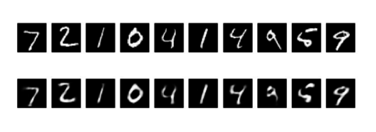

Input
Output
Now with this, we come to an end to this Autoencoders Tutorial. I Hope you guys enjoyed this article and understood the power of Tensorflow, and how easy it is to decompress images. So, if you have read this, you are no longer a newbie to Autoencoders. Try out these examples and let me know if there are any challenges you are facing while deploying the code.
Autoencoders Tutorial using TensorFlow | Edureka
This video provides you with a brief introduction about autoencoders and how they compress unsupervised data.

Check out this Artificial Intelligence Course by Edureka to upgrade your AI skills to the next level You will master concepts such as SoftMax function, Autoencoder Neural Networks, Restricted Boltzmann Machine (RBM) and work with libraries like Keras & TFLearn. Got a question for us? Please mention it in the comments section of “Autoencoders Tutorial” and we will get back to you.