Artificial Intelligence With Python: A Comprehensive Guide

Artificial Intelligence With Python:

Artificial Intelligence has been around for over half a century now and its advancements are growing at an exponential rate. The demand for AI is at its peak and if you wish to learn about Artificial Intelligence, you’ve landed at the right place. This blog on Artificial Intelligence With Python will help you understand all the concepts of AI with practical implementations in Python.

The following topics are covered in this Artificial Intelligence With Python blog:

1. Why Is Python Best For AI?
2. Demand For AI
3. What Is Artificial Intelligence?
4. Types Of Artificial Intelligence
5. Machine Learning Basics
6. Types Of Machine Learning
7. Types Of Problems Solved By Using Machine Learning
8. Machine Learning Process
9. Machine Learning With Python
10. Limitations Of Machine Learning
11. Why Deep Learning?
12. How Deep Learning Works?
13. What Is Deep Learning?
14. Deep Learning Use Case
15. Perceptrons
16. Multilayer Perceptrons
17. Deep Learning With Python
18. Introduction To Natural Language Processing (NLP)
19. NLP Applications
20. Terminologies In NLP

Why Is Python Best For AI?

A lot of people have asked me, ‘Which programming language is best for AI?’ or “Why Python for AI?”

Despite being a general purpose language, Python has made its way into the most complex technologies such as Artificial Intelligence, Machine Learning, Deep Learning, and so on. Having a Python programming certification is like having the upperhand advantage when compared with other developers who don’t have it.

Why has Python gained so much popularity in all these fields?

Here is a list of reasons why Python is the choice of language for every core Developer, Data Scientist, Machine Learning Engineer, etc:

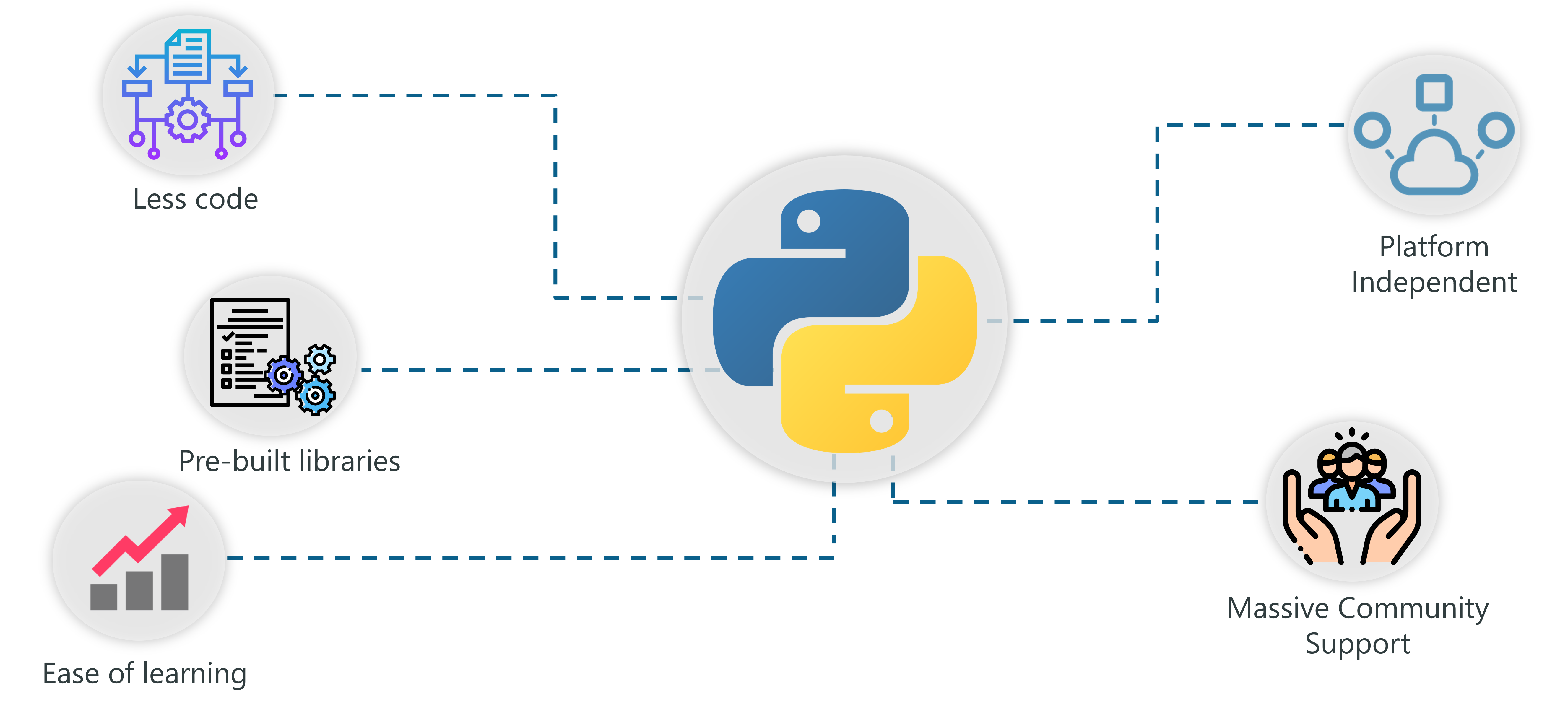
Why Python For AI – Artificial Intelligence With Python – Edureka

• Less Code: Implementing AI involves tons and tons of algorithms. Thanks to Pythons support for pre-defined packages, we don’t have to code algorithms. And to make things easier, Python provides “check as you code” methodology that reduces the burden of testing the code.
• Prebuilt Libraries: Python has 100s of pre-built libraries to implement various Machine Learning and Deep Learning algorithms. So every time you want to run an algorithm on a data set, all you have to do is install and load the necessary packages with a single command. Examples of pre-built libraries include NumPy, Keras, Tensorflow, Pytorch, and so on.
• Ease of learning: Python uses a very simple syntax that can be used to implement simple computations like, the addition of two strings to complex processes such as building a Machine Learning model.
• Platform Independent: Python can run on multiple platforms including Windows, MacOS, Linux, Unix, and so on. While transferring code from one platform to the other you can make use of packages such as PyInstaller that will take care of any dependency issues.
• Massive Community Support: Python has a huge community of users which is always helpful when we encounter coding errors. Apart from a huge fan following, Python has multiple communities, groups, and forums where programmers post their errors and help each other.

If you wish to learn Python Programming in depth, here are a couple of links to our other blog posts, do give those a read:

1. Python Tutorial – A Complete Guide to Learn Python Programming
2. Python Programming Language – Headstart With Python Basics
3. A Beginners Guide To Python Functions
4. Python for Data Science

Since this blog is all about Artificial Intelligence With Python, I will introduce you to the most effective and popular AI-based Python Libraries.

1. Tensorflow: Developed by Google, this library is popularly used in writing Machine Learning algorithms and performing heavy computations that involve Neural Networks.
2. Scikit-Learn: Scikit-learn is a Python library associated with NumPy and SciPy. It is considered as one of the best libraries for working with complex data.
3. NumPy: Numpy is a python library specifically used for computing scientific/mathematical data.
4. Theano: Theano is a functional library that effectively calculates and computes mathematical expressions involving multi-dimensional arrays.
5. Keras: This library simplifies the implementation of neural networks. It also has the best functionalities for computing models, evaluating data-sets, visualizing graphs, and much more.
6. NLTK: NLTK or Natural Language ToolKit is an open source Python library specifically built for Natural Language Processing, text analysis, and text mining.

In addition to the above-mentioned libraries make sure you check out Edureka’s blog post on Top 10 Python libraries to get a more clear understanding.

Now that you know the important Python libraries that are used for implementing AI techniques, let’s focus on Artificial Intelligence. In the next section, I will cover all the fundamental concepts of AI.

First, let’s start by understanding the sudden demand for AI.

Demand For AI

Since the emergence of AI in the 1950s, we have seen exponential growth in it’s potential. But if AI has been here for over half a century, why has it suddenly gained so much importance? Why are we talking about Artificial Intelligence now?

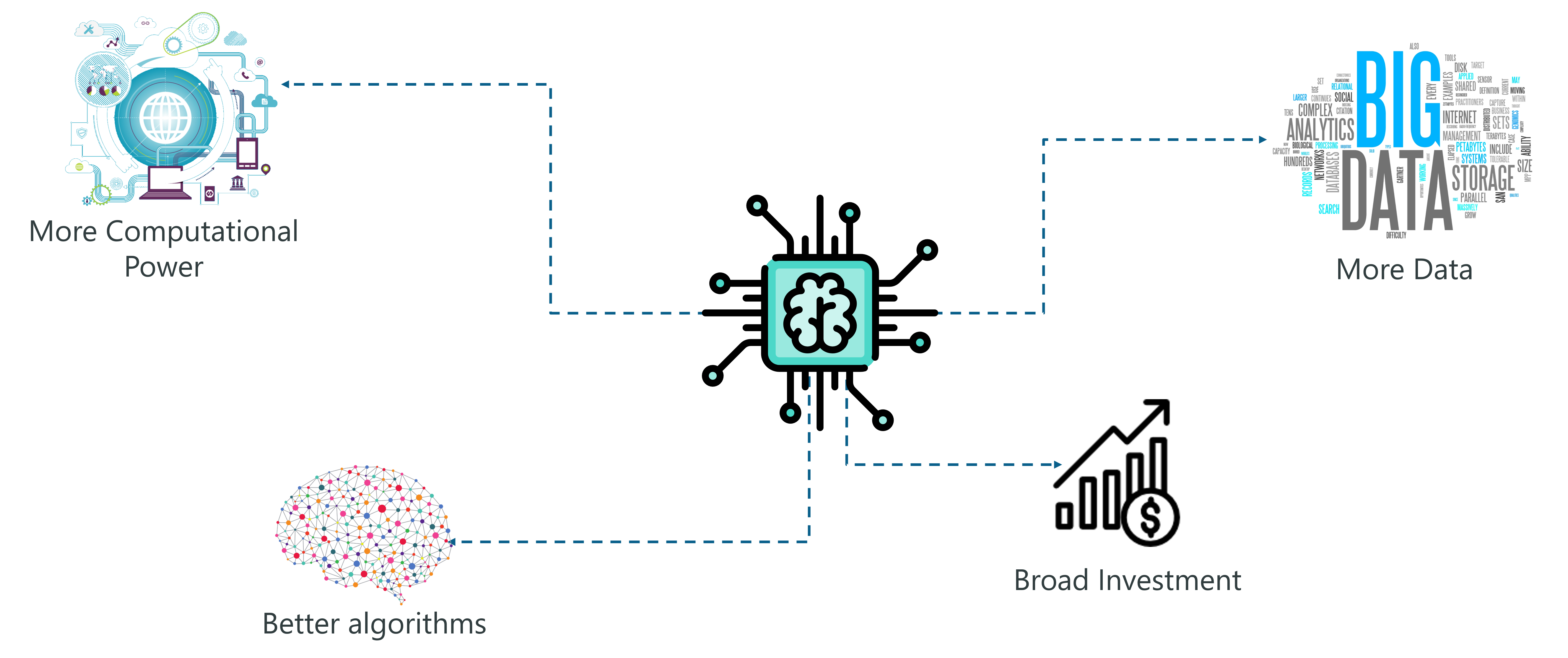
Demand For AI – Artificial Intelligence With Python – Edureka

The main reasons for the vast popularity of AI are:

More computing power: Implementing AI requires a lot of computing power since building AI models involve heavy computations and the use of complex neural networks. The invention of GPUs has made this possible. We can finally perform high-level computations and implement complex algorithms.

Data Generation: Over the past years, we’ve been generating an immeasurable amount of data. Such data needs to be analyzed and processed by using Machine Learning algorithms and other AI techniques.

More Effective Algorithms: In the past decade we’ve successfully managed to develop state of the art algorithms that involve the implementation of Deep Neural Networks.

Broad Investment: As tech giants such as Tesla, Netflix and Facebook started investing in Artificial Intelligence, it gained more popularity which led to an increase in the demand for AI-based systems.

The growth of Artificial Intelligence is exponential, it is also adding to the economy at an accelerated pace. So this is the right time for you to get into the field of Artificial Intelligence.

If you want to fast forward your career in AIML, then take up these Artificial Intelligence course by Edureka that offers LIVE instructor-led training, real-time projects, and certification.

What Is Artificial Intelligence?

The term Artificial Intelligence was first coined decades ago in the year 1956 by John McCarthy at the Dartmouth conference. He defined AI as:

“The science and engineering of making intelligent machines.”

In other words, Artificial Intelligence is the science of getting machines to think and make decisions like humans.

In the recent past, AI has been able to accomplish this by creating machines and robots that have been used in a wide range of fields including healthcare, robotics, marketing, business analytics and many more.

Now let’s discuss the different stages of Artificial Intelligence.

Types Of Artificial Intelligence

AI is structured along three evolutionary stages:

1. Artificial Narrow Intelligence
2. Artificial General Intelligence
3. Artificial Super Intelligence

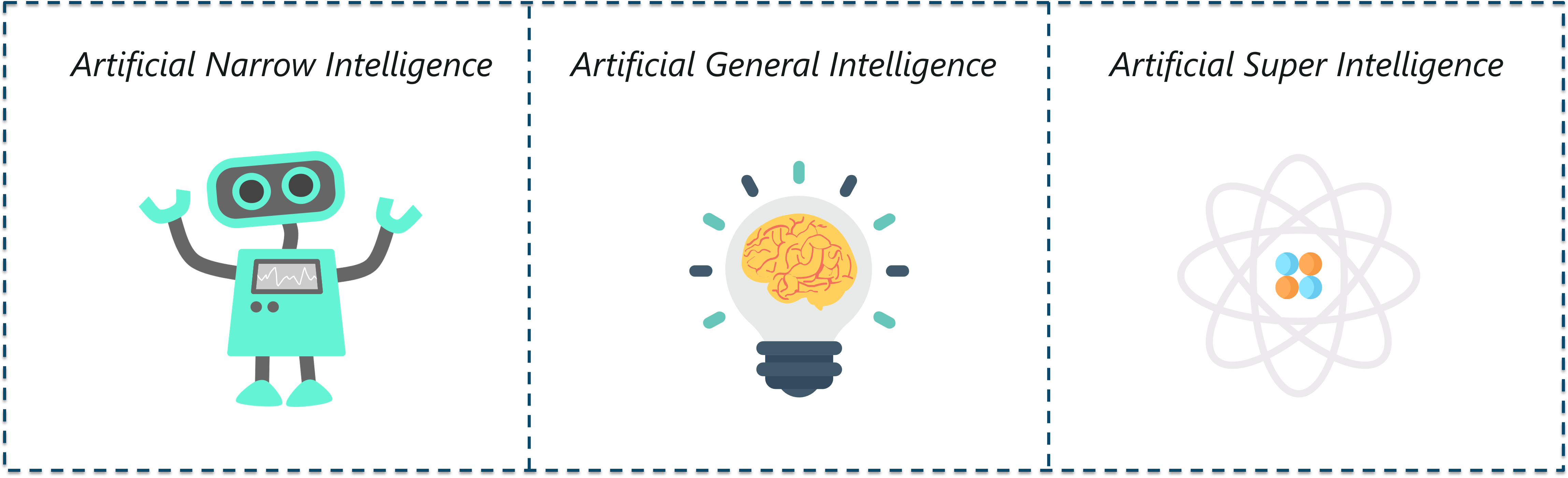
Types Of AI – Artificial Intelligence With Python – Edureka

Artificial Narrow Intelligence

Commonly known as weak AI, Artificial Narrow Intelligence involves applying AI only to specific tasks.

The existing AI-based systems that claim to use “artificial intelligence” are actually operating as a weak AI. Alexa is a good example of narrow intelligence. It operates within a limited predefined range of functions. Alexa has no genuine intelligence or self-awareness.

Google search engine, Sophia, self-driving cars and even the famous AlphaGo, fall under the category of weak AI.

Artificial General Intelligence

Commonly known as strong AI, Artificial General Intelligence involves machines that possess the ability to perform any intellectual task that a human being can.

You see, machines don’t possess human-like abilities, they have a strong processing unit that can perform high-level computations but they’re not yet capable of thinking and reasoning like a human.

There are many experts who doubt that AGI will ever be possible, and there are also many who question whether it would be desirable.

Stephen Hawking, for example, warned:

“Strong AI would take off on its own, and re-design itself at an ever-increasing rate. Humans, who are limited by slow biological evolution, couldn’t compete and would be superseded.”

Artificial Super Intelligence

Artificial Super Intelligence is a term referring to the time when the capability of computers will surpass humans.

ASI is presently seen as a hypothetical situation as depicted in movies and science fiction books, where machines have taken over the world. However, tech masterminds like Elon Musk believe that ASI will take over the world by 2040!

What do you think about Artificial Super Intelligence? Let me know your thoughts in the comment section.

Before I go any further, let me clear a very common misconception. I’ve been asked these question by every beginner:

What is the difference between AI and Machine Learning and Deep Learning?

Is AI the same as ML? 

Let’s break it down:

AI vs ML vs DL (Artificial Intelligence vs Machine Learning vs Deep Learning)

People tend to think that Artificial Intelligence, Machine Learning, and Deep Learning are the same since they have common applications. For example, Siri is an application of AI, Machine learning and Deep learning.

So how are these technologies related?

• Artificial Intelligence is the science of getting machines to mimic the behavior of humans.
• Machine learning is a subset of Artificial Intelligence (AI) that focuses on getting machines to make decisions by feeding them data.
• Deep learning is a subset of Machine Learning that uses the concept of neural networks to solve complex problems.

To sum it up AI, Machine Learning and Deep Learning are interconnected fields. Machine Learning and Deep learning aids Artificial Intelligence by providing a set of algorithms and neural networks to solve data-driven problems.

However, Artificial Intelligence is not restricted to only Machine learning and Deep learning. It covers a vast domain of fields including, Natural Language Processing (NLP), object detection, computer vision, robotics, expert systems and so on.

Now let’s get started with Machine Learning.

Machine Learning Basics

The term Machine Learning was first coined by Arthur Samuel in the year 1959. Looking back, that year was probably the most significant in terms of technological advancements.

In simple terms,

Machine learning is a subset of Artificial Intelligence (AI) which provides machines the ability to learn automatically by feeding it tons of data & allowing it to improve through experience. Thus, Machine Learning is a practice of getting Machines to solve problems by gaining the ability to think.

But how can a machine make decisions?

If you feed a machine a good amount of data, it will learn how to interpret, process and analyze this data by using Machine Learning Algorithms.

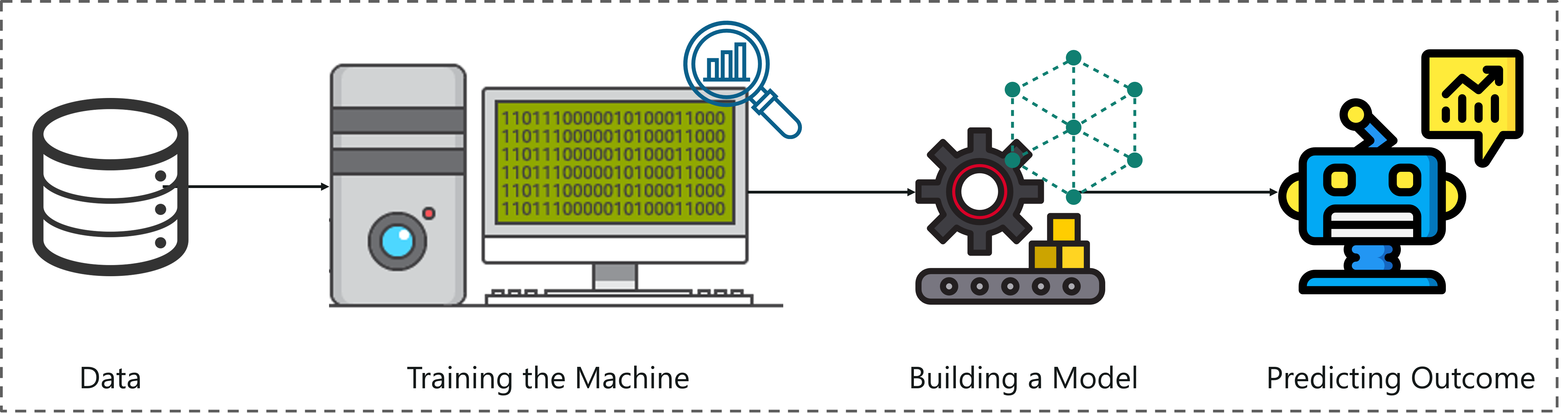
What Is Machine Learning – Artificial Intelligence With Python – Edureka

To sum it up, take a look at the above figure:

• A Machine Learning process begins by feeding the machine lots of data.
• The machine is then trained on this data, to detect hidden insights and patterns.
• These insights are used to build a Machine Learning Model by using an algorithm in order to solve a problem.

Now that we know what is Machine Learning, let’s look at the different ways in which machines can learn.

Types Of Machine Learning 

A machine can learn to solve a problem by following any one of the following three approaches:

1. Supervised Learning

2. Unsupervised Learning

3. Reinforcement Learning

Supervised Learning

Supervised learning is a technique in which we teach or train the machine using data which is well labeled.

To understand Supervised Learning let’s consider an analogy. As kids we all needed guidance to solve math problems. Our teachers helped us understand what addition is and how it is done.

Similarly, you can think of supervised learning as a type of Machine Learning that involves a guide. The labeled data set is the teacher that will train you to understand patterns in the data. The labeled data set is nothing but the training data set.

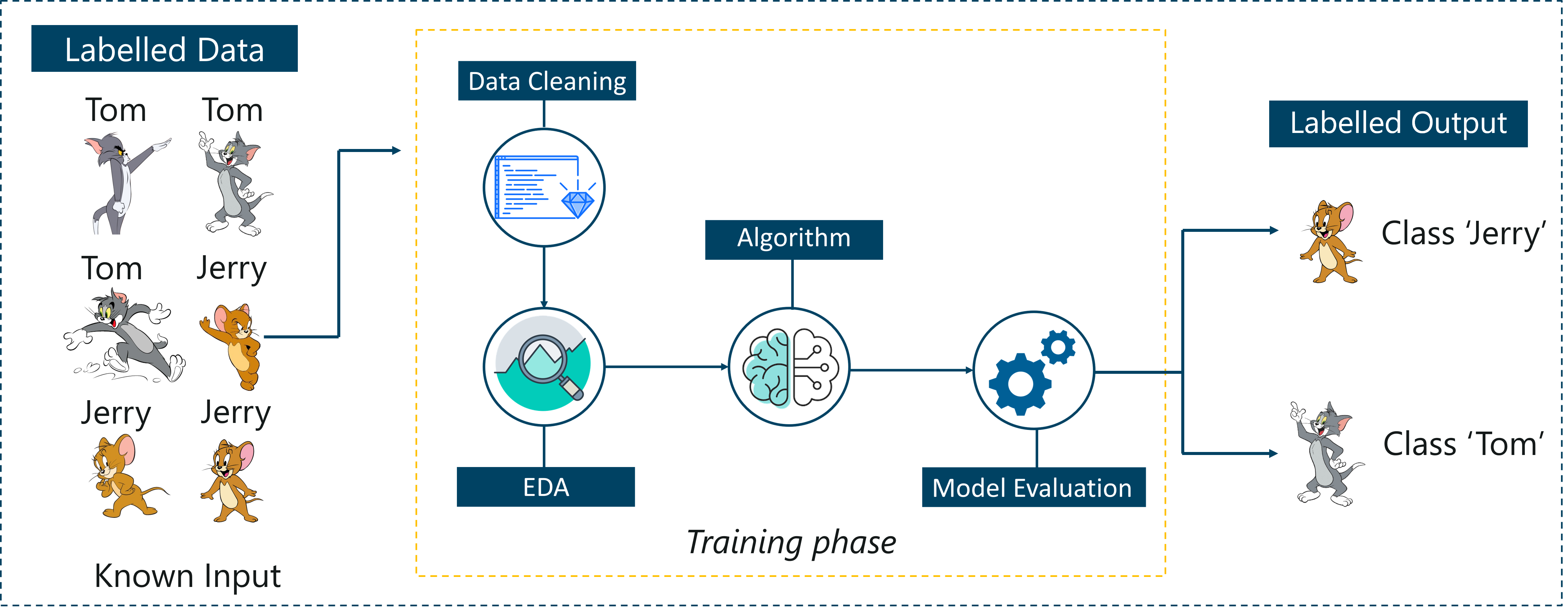Supervised Learning – Artificial Intelligence With Python – Edureka

Consider the above figure. Here we’re feeding the machine images of Tom and Jerry and the goal is for the machine to identify and classify the images into two groups (Tom images and Jerry images).

The training data set that is fed to the model is labeled, as in, we’re telling the machine, ‘this is how Tom looks and this is Jerry’. By doing so you’re training the machine by using labeled data. In Supervised Learning, there is a well-defined training phase done with the help of labeled data.

Unsupervised Learning

Unsupervised learning involves training by using unlabeled data and allowing the model to act on that information without guidance.

Think of unsupervised learning as a smart kid that learns without any guidance. In this type of Machine Learning, the model is not fed with labeled data, as in the model has no clue that ‘this image is Tom and this is Jerry’, it figures out patterns and the differences between Tom and Jerry on its own by taking in tons of data.

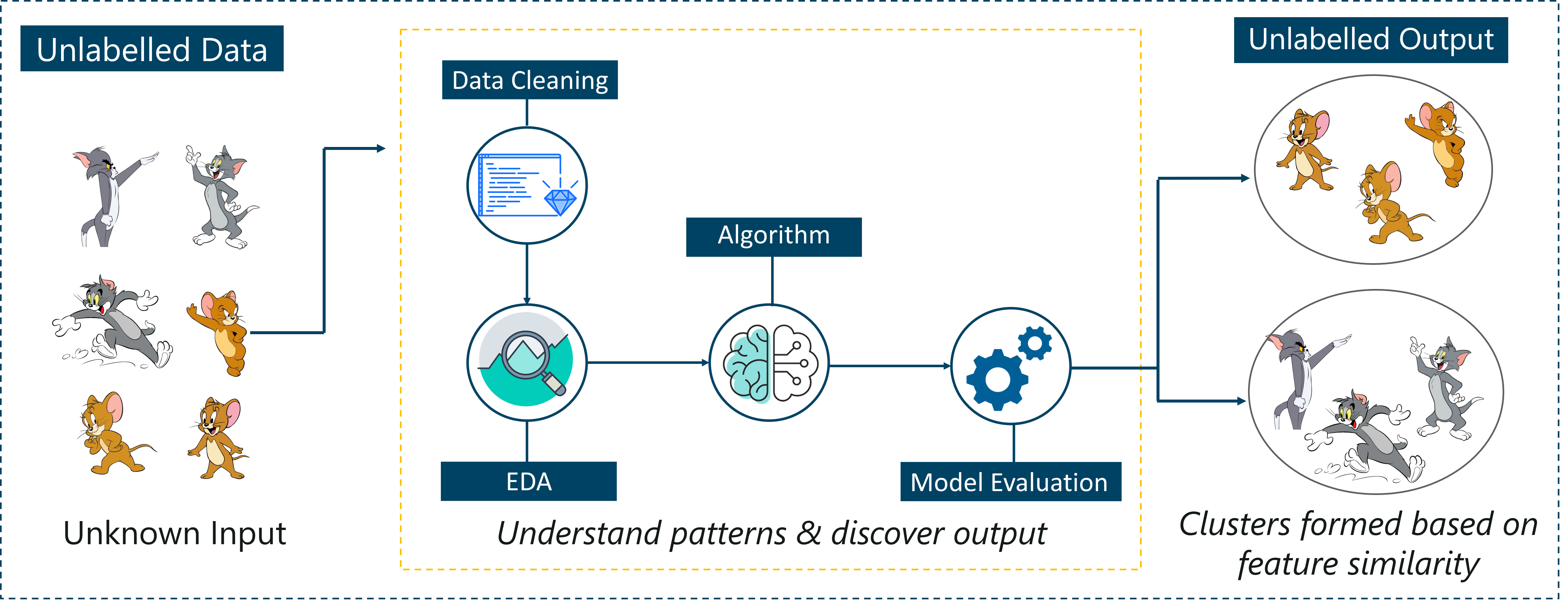Unsupervised Learning – Artificial Intelligence With Python – Edureka

For example, it identifies prominent features of Tom such as pointy ears, bigger size, etc, to understand that this image is of type 1. Similarly, it finds such features in Jerry and knows that this image is of type 2.

Therefore, it classifies the images into two different classes without knowing who Tom is or Jerry is.

Reinforcement Learning

Reinforcement Learning is a part of Machine learning where an agent is put in an environment and he learns to behave in this environment by performing certain actions and observing the rewards which it gets from those actions.

Imagine that you were dropped off at an isolated island!

What would you do?

Panic? Yes, of course, initially we all would. But as time passes by, you will learn how to live on the island. You will explore the environment, understand the climate condition, the type of food that grows there, the dangers of the island, etc.

This is exactly how Reinforcement Learning works, it involves an Agent (you, stuck on the island) that is put in an unknown environment (island), where he must learn by observing and performing actions that result in rewards.

Reinforcement Learning is mainly used in advanced Machine Learning areas such as self-driving cars, AplhaGo, etc. So that sums up the types of Machine Learning.

Now, let’s look at the type of problems that are solved by using Machine Learning.

What Problems Can Machine Learning Solve?

There are three main categories of problems that can be solved using Machine Learning:

What is Regression?

In this type of problem, the output is a continuous quantity. For example, if you want to predict the speed of a car given the distance, it is a Regression problem. Regression problems can be solved by using Supervised Learning algorithms like Linear Regression.

What is Classification?

In this type, the output is a categorical value. Classifying emails into two classes, spam and non-spam is a classification problem that can be solved by using Supervised Learning classification algorithms such as Support Vector Machines, Naive Bayes, Logistic Regression, K Nearest Neighbor, etc.

What is Clustering?

This type of problem involves assigning the input into two or more clusters based on feature similarity. For example, clustering viewers into similar groups based on their interests, age, geography, etc can be done by using Unsupervised Learning algorithms like K-Means Clustering.

Here’s a table that sums up the difference between Regression, Classification, and Clustering:

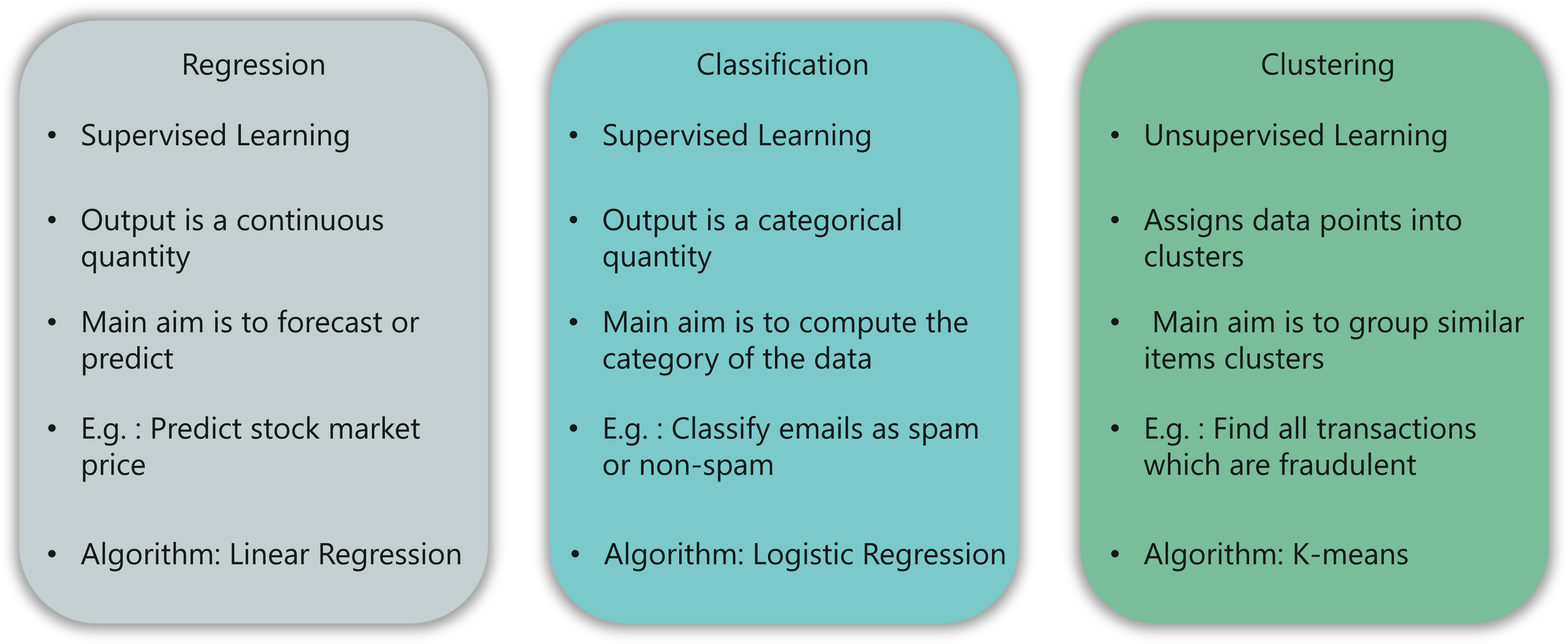
Regression vs Classification vs Clustering – Artificial Intelligence With Python – Edureka

Now let’s look at how the Machine Learning process works.

Machine Learning Process Steps

The Machine Learning process involves building a Predictive model that can be used to find a solution for a Problem Statement.

To understand the Machine Learning process let’s assume that you have been given a problem that needs to be solved by using Machine Learning.

The problem is to predict the occurrence of rain in your local area by using Machine Learning.

The below steps are followed in a Machine Learning process:

Step 1: Define the objective of the Problem Statement

At this step, we must understand what exactly needs to be predicted. In our case, the objective is to predict the possibility of rain by studying weather conditions.

It is also essential to take mental notes on what kind of data can be used to solve this problem or the type of approach you must follow to get to the solution.

Step 2: Data Gathering

At this stage, you must be asking questions such as,

• What kind of data is needed to solve this problem?
• Is the data available?
• How can I get the data?

Once you know the types of data that is required, you must understand how you can derive this data. Data collection can be done manually or by web scraping.

However, if you’re a beginner and you’re just looking to learn Machine Learning you don’t have to worry about getting the data. There are 1000s of data resources on the web, you can just download the data set and get going.

Coming back to the problem at hand, the data needed for weather forecasting includes measures such as humidity level, temperature, pressure, locality, whether or not you live in a hill station, etc.

Such data must be collected and stored for analysis.

Step 3: Data Preparation

The data you collected is almost never in the right format. You will encounter a lot of inconsistencies in the data set such as missing values, redundant variables, duplicate values, etc.

Removing such inconsistencies is very essential because they might lead to wrongful computations and predictions. Therefore, at this stage, you scan the data set for any inconsistencies and you fix them then and there.

Step 4: Exploratory Data Analysis

Grab your detective glasses because this stage is all about diving deep into data and finding all the hidden data mysteries.

EDA or Exploratory Data Analysis is the brainstorming stage of Machine Learning. Data Exploration involves understanding the patterns and trends in the data. At this stage, all the useful insights are drawn and correlations between the variables are understood.

For example, in the case of predicting rainfall, we know that there is a strong possibility of rain if the temperature has fallen low. Such correlations must be understood and mapped at this stage.

Step 5: Building a Machine Learning Model

All the insights and patterns derived during Data Exploration are used to build the Machine Learning Model. This stage always begins by splitting the data set into two parts, training data, and testing data.

The training data will be used to build and analyze the model. The logic of the model is based on the Machine Learning Algorithm that is being implemented.

In the case of predicting rainfall, since the output will be in the form of True (if it will rain tomorrow) or False (no rain tomorrow), we can use a Classification Algorithm such as Logistic Regression or Decision Tree.

Choosing the right algorithm depends on the type of problem you’re trying to solve, the data set and the level of complexity of the problem.

Step 6: Model Evaluation & Optimization

After building a model by using the training data set, it is finally time to put the model to a test.

The testing data set is used to check the efficiency of the model and how accurately it can predict the outcome.

Once the accuracy is calculated, any further improvements in the model can be implemented at this stage. Methods like parameter tuning and cross-validation can be used to improve the performance of the model.

Step 7: Predictions

Once the model is evaluated and improved, it is finally used to make predictions. The final output can be a Categorical variable (eg. True or False) or it can be a Continuous Quantity (eg. the predicted value of a stock).

In our case, for predicting the occurrence of rainfall, the output will be a categorical variable.

So that was the entire Machine Learning process.

In the next section, we will discuss the various types of Machine Learning Algorithms.

Machine Learning Algorithms

Machine Learning Algorithms are the basic logic behind each Machine Learning model. These algorithms are based on simple concepts such as Statistics and Probability.

Follow the below-mentioned blogs to understand the Math and stats behind Machine Learning Algorithms:

1. A Complete Guide To Math And Statistics For Data Science
2. All You Need To Know About Statistics And Probability

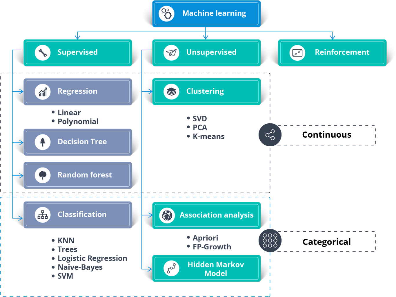
Machine Learning Algorithms – Artificial Intelligence With Python – Edureka

The above figure shows the different algorithms used to solve a problem using Machine Learning.

Supervised Learning can be used to solve two types of Machine Learning problems:

1. Regression
2. Classification

To solve Regression problems you can use the famous Linear Regression Algorithm. Here’s a Linear Regression Algorithm from Scratch blog that will help you understand how it works.

Classification problems can be solved using the following Classification Algorithms:

1. Logistic Regression
2. Decision Tree
3. Random Forest
4. Naive Bayes Classifier
5. Support Vector Machine
6. K Nearest Neighbour

Unsupervised Learning can be used to solve Clustering and association problems. One of the famous clustering algorithms is the K-means Clustering algorithm.

You can check out this video on K-means clustering to learn more about it.

Reinforcement Learning can be used to solve reward-based problems. The famous Q-learning Algorithm is commonly used to solve Reinforcement Learning problems.

Here’s a video on Reinforcement Learning that covers all the important concepts of Reinforcement Learning along with a practical implementation of Q-learning using Python.

Now to better understand the entire Machine Learning flow, let’s perform a practical implementation of Machine Learning using Python.

Machine Learning With Python

In this section, we will implement Machine Learning by using Python. So let’s begin.

Problem Statement: To build a Machine Learning model which will predict whether or not it will rain tomorrow by studying past data.

Data Set Description: This data set contains around 145k observations on the daily weather conditions as observed from numerous Australian weather stations. The data set has around 24 features and we will be using 23 features (Predictor variables) to predict the target variable, which is, “RainTomorrow”.

This target variable (RainTomorrow) will store two values:

1. Yes: Denotes that it will rain tomorrow
2. No: Denotes it will not rain tomorrow

Therefore, this is clearly a classification problem. The Machine Learning model will classify the output into 2 classes, either YES or NO.

Logic: To build Classification models in order to predict whether or not it will rain tomorrow based on the weather conditions.

Now that the objective is clear, let’s get our brains working and start coding.

Step 1: Import the required libraries

# For linear algebra
import numpy as np
# For data processing
import pandas as pd

Step 2: Load the data set 

#Load the data set
df = pd.read_csv('. . . Desktop/weatherAUS.csv')
#Display the shape of the data set
print('Size of weather data frame is :',df.shape)
#Display data
print(df[0:5])

Size of weather data frame is : (145460, 24)
        Date         Location   MinTemp ... RainToday  RISK_MM  RainTomorrow
0   2008-12-01   Albury           13.4 ...         No             0.0                   No
1   2008-12-02   Albury            7.4 ...          No             0.0                   No
2   2008-12-03   Albury          12.9 ...          No             0.0                   No
3   2008-12-04   Albury            9.2 ...          No             1.0                   No
4   2008-12-05   Albury          17.5 ...          No             0.2                   No

Step 3: Data Preprocessing

# Checking for null values
print(df.count().sort_values())

[5 rows x 24 columns]
Sunshine 75625
Evaporation 82670
Cloud3pm 86102
Cloud9am 89572
Pressure9am 130395
Pressure3pm 130432
WindDir9am 134894
WindGustDir 135134
WindGustSpeed 135197
Humidity3pm 140953
WindDir3pm 141232
Temp3pm 141851
RISK_MM 142193
RainTomorrow 142193
RainToday 142199
Rainfall 142199
WindSpeed3pm 142398
Humidity9am 142806
Temp9am 143693
WindSpeed9am 143693
MinTemp 143975
MaxTemp 144199
Location 145460
Date 145460
dtype: int64

Notice the output, it shows that the first four columns have more than 40% null values, therefore, it is best if we get rid of these columns.

During data preprocessing it is always necessary to remove the variables that are not significant. Unnecessary data will just increase our computations. Therefore we will remove the ‘location’ variable and the ‘date’ variable since they’re not significant for predicting the weather.

We will also remove the ‘RISK_MM’ variable because we want to predict ‘RainTomorrow’ and RISK_MM (amount of rain the next day) can leak some info to our model.

df = df.drop(columns=['Sunshine','Evaporation','Cloud3pm','Cloud9am','Location','RISK_MM','Date'],axis=1)
print(df.shape)

(145460, 17)

Next, we will remove all the null values in our data frame.

#Removing null values
df = df.dropna(how='any')
print(df.shape)

(112925, 17)

After removing null values, we must also check our data set for any outliers. An outlier is a data point that significantly differs from other observations. Outliers usually occur due to miscalculations while collecting the data.

In the below code snippet we’re getting rid of outliers:

from scipy import stats
z = np.abs(stats.zscore(df._get_numeric_data()))
print(z)
df= df[(z < 3).all(axis=1)]
print(df.shape)

[[0.11756741 0.10822071 0.20666127 ... 1.14245477 0.08843526 0.04787026]
[0.84180219 0.20684494 0.27640495 ... 1.04184813 0.04122846 0.31776848]
[0.03761995 0.29277194 0.27640495 ... 0.91249673 0.55672435 0.15688743]
...
[1.44940294 0.23548728 0.27640495 ... 0.58223051 1.03257127 0.34701958]
[1.16159206 0.46462594 0.27640495 ... 0.25166583 0.78080166 0.58102838]
[0.77784422 0.4789471 0.27640495 ... 0.2085487 0.37167606 0.56640283]]
(107868, 17)

Next, we’ll be assigning ‘0s’ and ‘1s’ in the place of ‘YES’ and ‘NO’.

#Change yes and no to 1 and 0 respectvely for RainToday and RainTomorrow variable
df['RainToday'].replace({'No': 0, 'Yes': 1},inplace = True)
df['RainTomorrow'].replace({'No': 0, 'Yes': 1},inplace = True)

Now it’s time normalise the data in order to avoid any baissness while predicting the outcome. To do this, we can make use of the MinMaxScaler function that is present in the sklearn library.

from sklearn import preprocessing
scaler = preprocessing.MinMaxScaler()
scaler.fit(df)
df = pd.DataFrame(scaler.transform(df), index=df.index, columns=df.columns)
df.iloc[4:10]

MinTemp  MaxTemp  Rainfall  ...  WindDir9am_W  WindDir9am_WNW  WindDir9am_WSW
4   0.628342  0.696296    0.035714 ...         0.0                 0.0                                        0.0
5   0.550802  0.632099    0.007143 ...         1.0                 0.0                                        0.0
6   0.542781  0.516049    0.000000 ...         0.0                 0.0                                        0.0
7   0.366310  0.558025    0.000000 ...         0.0                 0.0                                        0.0
8   0.419786  0.686420    0.000000 ...         0.0                 0.0                                        0.0
9   0.510695  0.641975    0.050000 ...         0.0                 0.0                                        0.0

[6 rows x 62 columns]

Step 4: Exploratory Data Analysis (EDA)

Now that we’re done pre-processing the data set, it’s time to check perform analysis and identify the significant variables that will help us predict the outcome. To do this we will make use of the SelectKBest function present in the sklearn library:

#Using SelectKBest to get the top features!
from sklearn.feature_selection import SelectKBest, chi2
X = df.loc[:,df.columns!='RainTomorrow']
y = df[['RainTomorrow']]
selector = SelectKBest(chi2, k=3)
selector.fit(X, y)
X_new = selector.transform(X)
print(X.columns[selector.get_support(indices=True)])

Index(['Rainfall', 'Humidity3pm', 'RainToday'], dtype='object')

The output gives us the three most significant predictor variables:

1. Rainfall

2. Humidity3pm

3. RainToday

The main aim of this demo is to make you understand how Machine Learning works, therefore, to simplify the computations we will assign only one of these significant variables as the input.

#The important features are put in a data frame
df = df[['Humidity3pm','Rainfall','RainToday','RainTomorrow']]

#To simplify computations we will use only one feature (Humidity3pm) to build the model

X = df[['Humidity3pm']]
y = df[['RainTomorrow']]

In the above code snippet, ‘X’ and ‘y’ denote the input and the output respectively.

Step 5: Building a Machine Learning Model

At this step, we will build the Machine Learning model by using the training data set and evaluate the efficiency of the model by using the testing data set.

We’ll be building classification models, by using the following algorithms:

1. Logistic Regression
2. Random Forest
3. Decision Tree
4. Support Vector Machine

Below is the code snippet for each of these classification models:

Logistic Regression

#Logistic Regression
from sklearn.linear_model import LogisticRegression
from sklearn.model_selection import train_test_split
from sklearn.metrics import accuracy_score
import time

#Calculating the accuracy and the time taken by the classifier
t0=time.time()
#Data Splicing
X_train,X_test,y_train,y_test = train_test_split(X,y,test_size=0.25)
clf_logreg = LogisticRegression(random_state=0)
#Building the model using the training data set
clf_logreg.fit(X_train,y_train)

#Evaluating the model using testing data set
y_pred = clf_logreg.predict(X_test)
score = accuracy_score(y_test,y_pred)

#Printing the accuracy and the time taken by the classifier
print('Accuracy using Logistic Regression:',score)
print('Time taken using Logistic Regression:' , time.time()-t0)

Accuracy using Logistic Regression: 0.8330181332740015
Time taken using Logistic Regression: 0.1741015911102295

Random Forest Classifier

#Random Forest Classifier
from sklearn.ensemble import RandomForestClassifier
from sklearn.model_selection import train_test_split

#Calculating the accuracy and the time taken by the classifier
t0=time.time()
#Data Splicing
X_train,X_test,y_train,y_test = train_test_split(X,y,test_size=0.25)
clf_rf = RandomForestClassifier(n_estimators=100, max_depth=4,random_state=0)
#Building the model using the training data set
clf_rf.fit(X_train,y_train)

#Evaluating the model using testing data set
y_pred = clf_rf.predict(X_test)
score = accuracy_score(y_test,y_pred)

#Printing the accuracy and the time taken by the classifier
print('Accuracy using Random Forest Classifier:',score)
print('Time taken using Random Forest Classifier:' , time.time()-t0)

Accuracy using Random Forest Classifier: 0.8358363926280269
Time taken using Random Forest Classifier: 3.7179694175720215

Decision Tree Classifier

#Decision Tree Classifier
from sklearn.tree import DecisionTreeClassifier
from sklearn.model_selection import train_test_split

#Calculating the accuracy and the time taken by the classifier
t0=time.time()
#Data Splicing
X_train,X_test,y_train,y_test = train_test_split(X,y,test_size=0.25)
clf_dt = DecisionTreeClassifier(random_state=0)
#Building the model using the training data set
clf_dt.fit(X_train,y_train)

#Evaluating the model using testing data set
y_pred = clf_dt.predict(X_test)
score = accuracy_score(y_test,y_pred)

#Printing the accuracy and the time taken by the classifier
print('Accuracy using Decision Tree Classifier:',score)
print('Time taken using Decision Tree Classifier:' , time.time()-t0)

Accuracy using Decision Tree Classifier: 0.831423591797382
Time taken using Decision Tree Classifier: 0.0849456787109375

Support Vector Machine

#Support Vector Machine
from sklearn import svm
from sklearn.model_selection import train_test_split

#Calculating the accuracy and the time taken by the classifier
t0=time.time()
#Data Splicing
X_train,X_test,y_train,y_test = train_test_split(X,y,test_size=0.25)
clf_svc = svm.SVC(kernel='linear')

#Building the model using the training data set
clf_svc.fit(X_train,y_train)

#Evaluating the model using testing data set
y_pred = clf_svc.predict(X_test)
score = accuracy_score(y_test,y_pred)

#Printing the accuracy and the time taken by the classifier
print('Accuracy using Support Vector Machine:',score)
print('Time taken using Support Vector Machine:' , time.time()-t0)

Accuracy using Support Vector Machine: 0.7886676308080246
Time taken using Support Vector Machine: 88.42247271537781

All the classification models give us an accuracy score of approximately 83-84 % except for Support Vector Machines. Considering the size of our data set, the accuracy is pretty good.

So give yourself a pat on the back because you now know how to solve problems by using Machine Learning.

To learn more about Machine Learning, give these blogs a read:

1. What is Machine Learning? Machine Learning For Beginners
2. Machine Learning Tutorial for Beginners
3. Latest Machine Learning Projects to Try in 2024

Now let’s look at a more advanced concept called Deep Learning.

Before we understand what Deep Learning is, let’s understand the limitations of Machine Learning. These limitations gave rise to the concept of Deep Learning.

Limitations Of Machine Learning

The following are the limitations of Machine Learning:

1. Machine Learning is not capable of handling and processing high dimensional data.
2. It cannot be used in image recognition and object detection since they require the implementation of high dimensional data
3. Another major challenge in Machine Learning is to tell the machine what are the important features it should look for in order to precisely predict the outcome. This very process is called feature extraction. Feature extraction is a manual process in Machine Learning.

The above limitations can be solved by using Deep Learning.

Why Deep Learning?

• Deep learning is one of the only methods by which we can overcome the challenges of feature extraction. This is because deep learning models are capable of learning to focus on the right features by themselves, requiring minimal human interventions.

• Deep Learning is mainly used to deal with high dimensional data. It is based o the concept of Neural Networks and is often used in object detection and image processing.

Now let’s understand how Deep Learning works.

How Deep Learning Works?

Deep Learning mimics the basic component of the human brain called a brain cell or a neuron. Inspired from a neuron an artificial neuron was developed.

Deep Learning is based on the functionality of a biological neuron, so let’s understand how we mimic this functionality in the artificial neuron (also known as a perceptron):

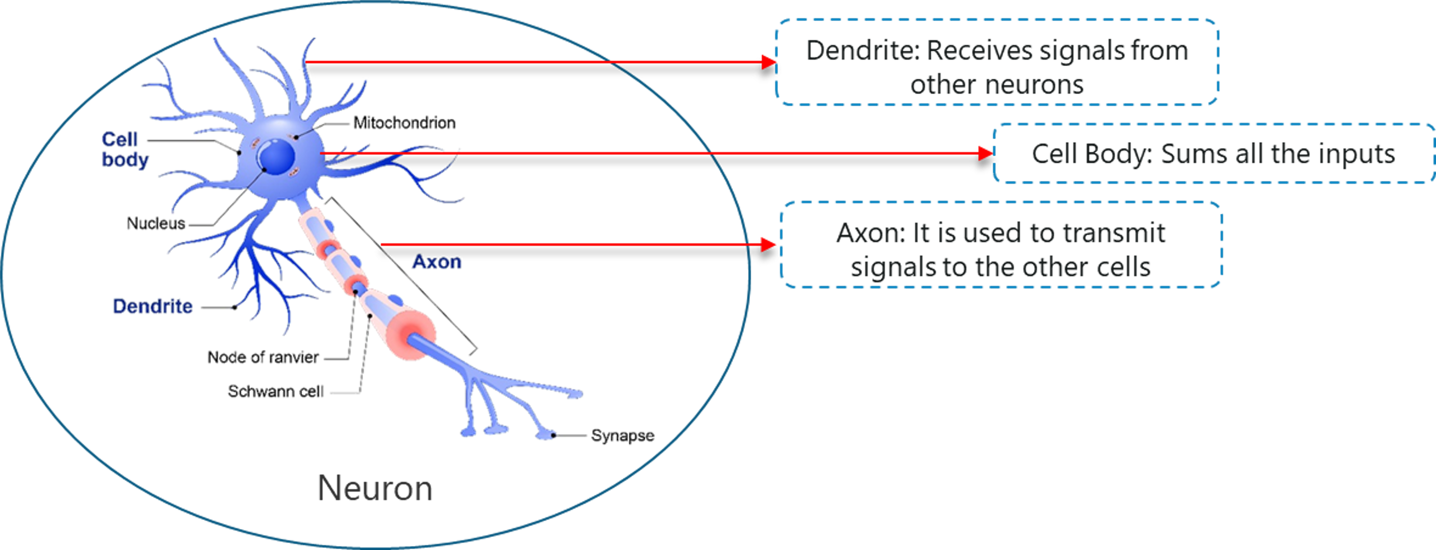
Biological Neuron – Artificial Intelligence With Python – Edureka

• In a biological neuron, dendrites are used to receive inputs. These inputs are summed in the cell body and through the Axon, it is passed on to the next neuron.
• Similar to the biological neuron, a perceptron receives multiple inputs, applies various transformations and functions and provides an output.
• The human brain consists of multiple connected neurons called a neural network, similarly, by combining multiple perceptrons, we’ve developed what is known as a Deep neural network.

Now let’s understand what exactly Deep Learning is.

What Is Deep Learning?

“Deep Learning is a collection of statistical machine learning techniques used to learn feature hierarchies based
on the concept of artificial neural networks.”

A Deep neural network consists of the following layers:

1. The Input Layer
2. The Hidden Layer
3. The Output Layer

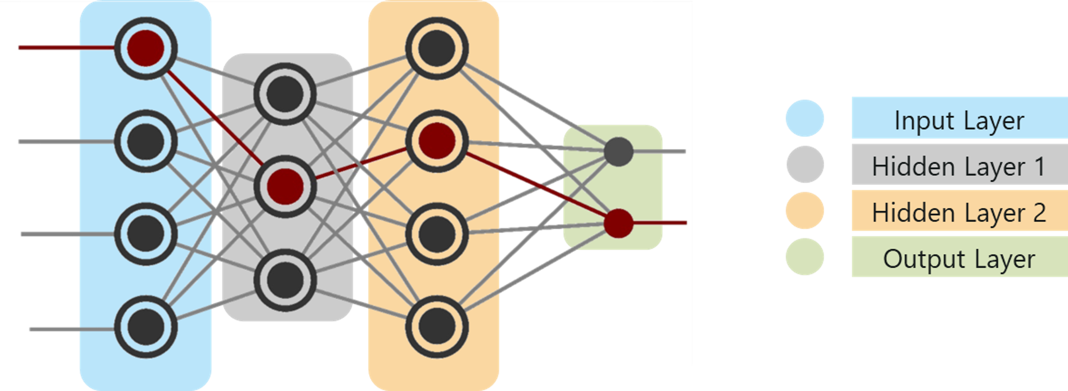
What Is Deep Learning – Artificial Intelligence With Python – Edureka

In the above figure,

• The first layer is the input layer which receives all the inputs
• The last layer is the output layer which provides the desired output
• All the layers in between these layers are called hidden layers.
• There can be n number of hidden layers and the number of hidden layers and the number of perceptrons in each layer will entirely depend on the use-case you are trying to solve.

Deep Learning is used in highly computational use cases such as Face Verification, self-driving cars, and so on. Let’s understand the importance of Deep Learning by looking at a real-world use case.

Deep Learning Use Case

Consider how PayPal uses Deep Learning to identify any possible fraudulent activities. PayPal processed over $235 billion in payments from four billion transactions by its more than 170 million customers.

PayPal used Machine learning and Deep Learning algorithms to mine data from the customer’s purchasing history in addition to reviewing patterns of likely fraud stored in its databases to predict whether a particular transaction is fraudulent or not.

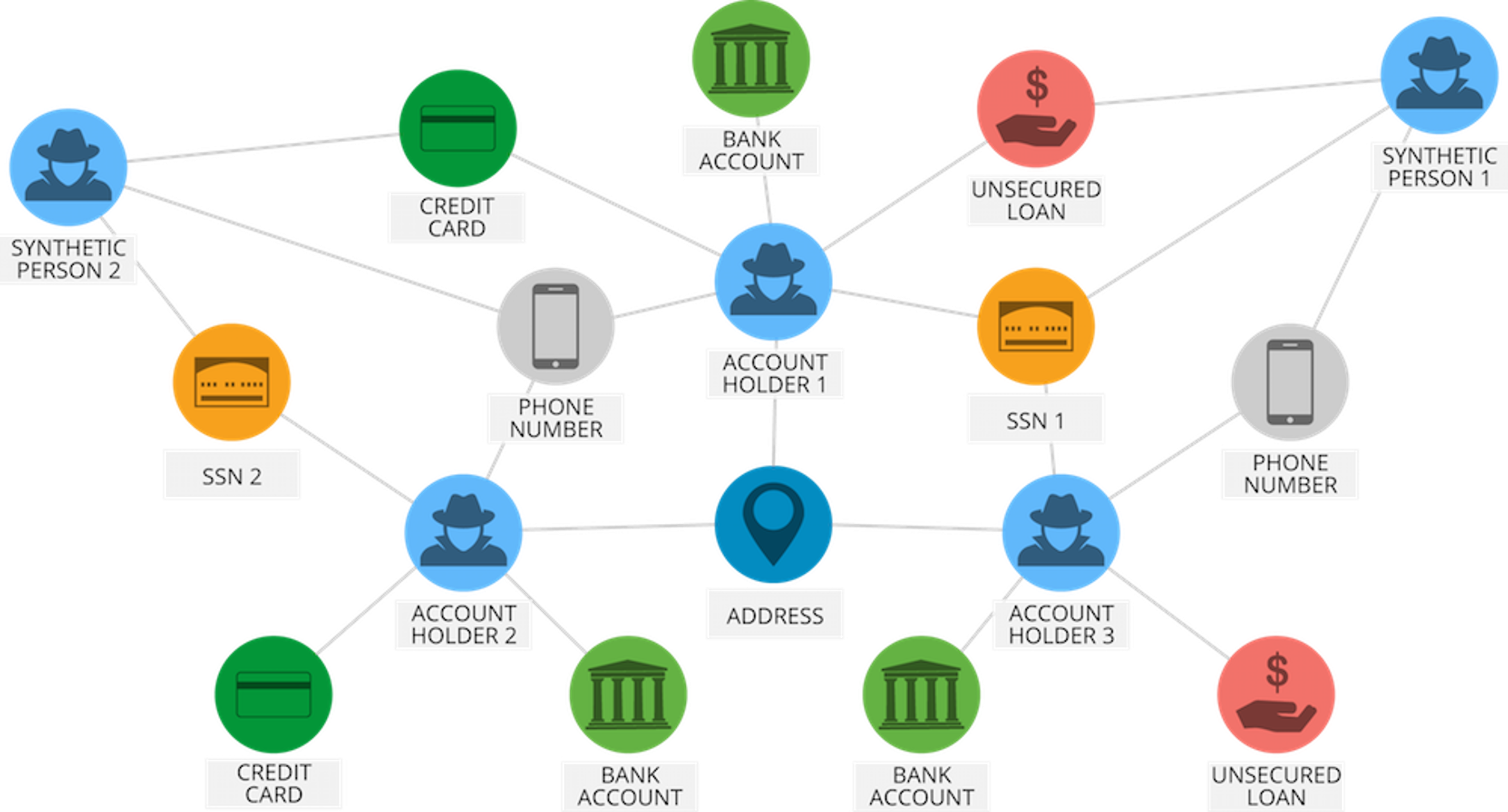
Deep Learning Use Case – Artificial Intelligence With Python – Edureka

The company has been relying on Deep Learning & Machine Learning technology for around 10 years. Initially, the fraud monitoring team used simple, linear models. But over the years the company switched to a more advanced Machine Learning technology called, Deep Learning.

Fraud risk manager and Data Scientist at PayPal, Ke Wang, quoted:

“What we enjoy from more modern, advanced machine learning is its ability to consume a lot more data, handle layers and layers of abstraction and be able to ‘see’ things that a simpler technology would not be able to see, even human beings might not be able to see.”

A simple linear model is capable of consuming around 20 variables. However, with Deep Learning technology one can run thousands of data points.

“There’s a magnitude of difference — you’ll be able to analyze a lot more information and identify patterns that are a lot more sophisticated,” Ke Wang said.

Therefore, by implementing Deep Learning technology, PayPal can finally analyze millions of transactions to identify any fraudulent activity.

To better understand Deep Learning, let’s understand how a Perceptron works.

What Is A Perceptron?

A Perceptron is a single layer neural network that is used to classify linear data. The perceptron has 4 important components:

1. Input
2. Weights and Bias
3. Summation Function
4. Activation or transformation Function

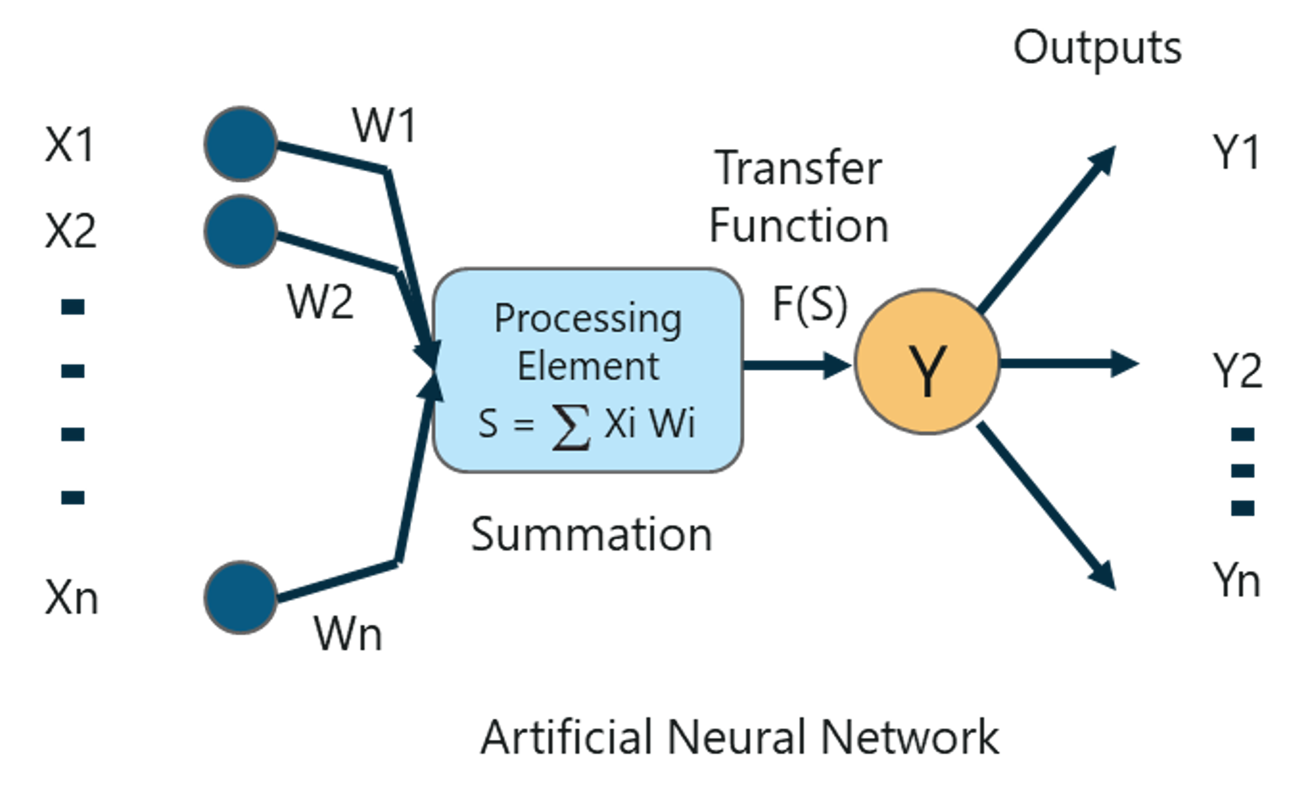
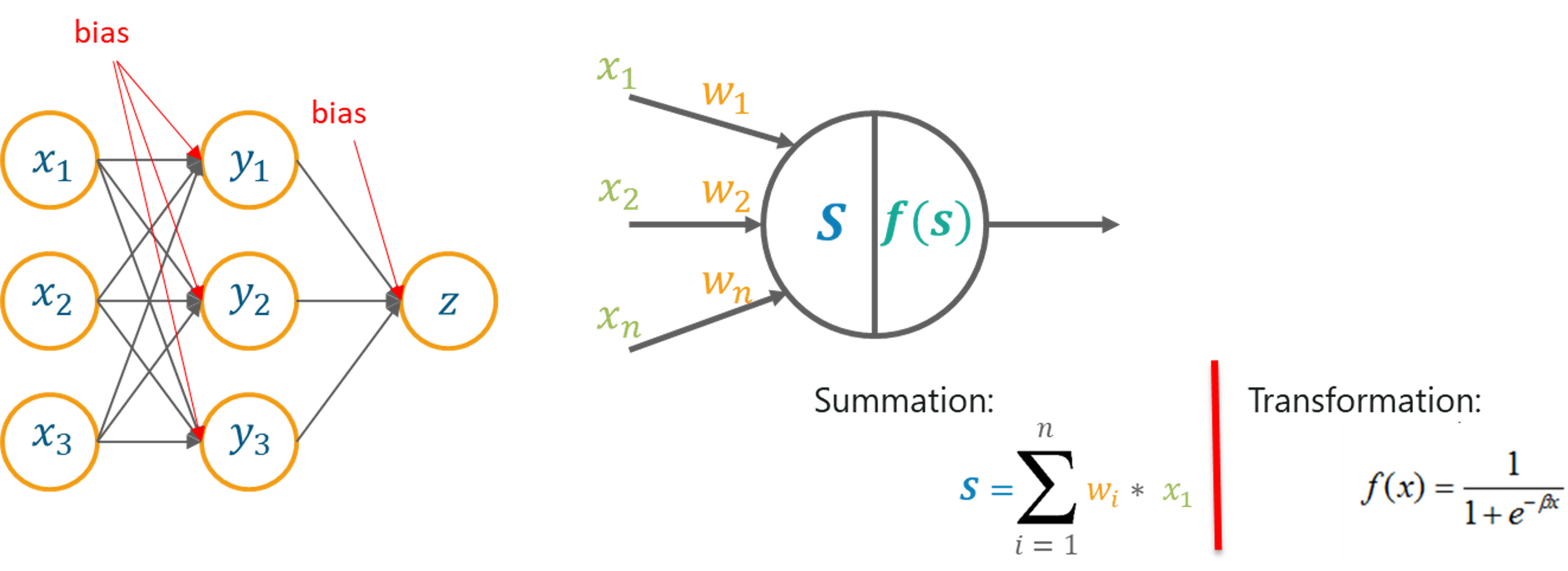
Perceptron – Artificial Intelligence With Python – Edureka

The basic logic behind a perceptron is as follows:

The inputs (x) received from the input layer are multiplied with their assigned weights w.  The multiplied values are then added to form the Weighted Sum. The weighted sum of the inputs and their respective weights are then applied to a relevant Activation Function. The activation function maps the input to the respective output.

Weights and Bias In Deep Learning

Why do we have to assign weights to each input?

Once an input variable is fed to the network, a randomly chosen value is assigned as the weight of that input. The weight of each input data point indicates how important that input is in predicting the outcome.

The bias parameter, on the other hand, allows you to adjust the activation function curve in such a way that a precise output is achieved.

Summation Function

Once the inputs are assigned some weight, the product of the respective input and weight is taken. Adding all these products gives us the Weighted Sum. This is done by the summation function.

Activation Function

The main aim of the activation functions is to map the weighted sum to the output. Activation functions such as tanh, ReLU, sigmoid and so on are examples of transformation functions.

To learn more about the functions of Perceptrons, you can go through this Deep Learning: Perceptron Learning Algorithm blog.

Now let’s understand the concept of Multilayer Perceptrons.

Why Multilayer Perceptron Is Used?

Single layer Perceptrons are not capable of handling high dimensional data and they can’t be used to classify non-linearly separable data.

Therefore, complex problems, that involve a large number of parameters can be solved by using Multilayer Perceptrons.

What Is A Multilayer Perceptron?

A Multilayer perceptron is a classifier that contains one or more hidden layers and it is based on the Feedforward artificial neural network. In the Feedforward networks, each neural network layer is fully connected to the following layer.

Multi-layer Perceptron – Artificial Intelligence With Python – Edureka

How does Multilayer Perceptron Work?

In a Multilayer Perceptron, the weights assigned to each input at the beginning are updated in order to minimize the resultant error in computation.

This is done because initially we randomly assign weight values for each input, these weight values obviously do not give us the desired outcome, therefore it is necessary to update the weights in such a manner that the output is precise.

This process of updating the weights and training the networks is known as Backpropagation.

Backpropagation is the logic behind Multilayer Perceptrons. This method is used to update the weights in such a way that the most significant input variable gets the maximum weight, thus reducing the error while computing the output.

So that was the logic behind Artificial Neural Networks. If you wish to learn more, make sure you give this, Neural Network Tutorial – Multi-Layer Perceptron blog a read.

Deep Learning With Python

To summarise how Deep Learning works, let’s look at an implementation of Deep Learning with Python.

Problem Statement: To study a bank credit data set and determine whether a transaction is fraudulent or not based on past data.

Data Set Description: The data set describes the transactions made by European cardholders in the years 2013. It contains transactional details of two days, where there are 492 fraudulent activities out of 284,807 transactions.

Logic: To build a Neural Network that can classify a transaction as either fraudulent or not based on past transactions.

Now that you know the objective of this demo, let’s get on with the demo.

Step 1: Import the necessary packages

#Import requires packages

import numpy as np
import pandas as pd
import os
os.environ["TF_CPP_MIN_LOG_LEVEL"]="3"
from sklearn.utils import shuffle
import matplotlib.pyplot as plt

# Import Keras, Dense, Dropout
from keras.models import Sequential
from keras.layers import Dense
from keras.layers import Dropout

import matplotlib.pyplot as plt
import seaborn as sns
from sklearn.preprocessing import MinMaxScaler
from sklearn.metrics import accuracy_score, precision_score, recall_score, f1_score
, fbeta_score, classification_report, confusion_matrix, precision_recall_curve, roc_auc_score
, roc_curve

Step 2: Load the data set

# Import the dataset
df_full = pd.read_csv('C://Users//NeelTemp//Desktop//ai with python//creditcard.csv')

# Print out first 5 row of the data set
print(df_full.head(5))

    Time          V1                V2            V3          ...    V27              V28         Amount    Class
0    0.0    -1.359807     -0.072781    2.536347    ... 0.133558    -0.021053      149.62        0
1    0.0     1.191857       0.266151    0.166480   ... -0.008983     0.014724      2.69            0
2    1.0    -1.358354     -1.340163    1.773209   ... -0.055353    -0.059752      378.66        0
3    1.0    -0.966272     -0.185226    1.792993   ... 0.062723      0.061458      123.50         0
4    2.0    -1.158233      0.877737    1.548718   ... 0.219422      0.215153      69.99           0

In the above description, the target varible is the ‘Class’ variable. It can hold two values:

1. Class 0: Denotes that the transaction is not fraudulent
2. Class 1: Denotes that the transaction is fraudulent

The rest of the variables are predictor variables that will help us understand whether or not a transaction is fraudulent.

# Count the number of samples for each class (Class 0 and Class 1)
print(df_full.Class.value_counts())

0   284315
1   492

Name: Class, dtype: int64

The above output shows that we have around 284k non-fraudulent transactions and ‘492’ fraudulent transactions. The difference between the two classes is huge and this makes our data set highly unbalanced. Therefore, we must sample out our dataset in such a way that the number of fraudulent to non-fraudulent transactions is balanced.

For this, we can make use of a statistical sampling technique called Stratified Sampling.

Step 3: Data Preperation

#Sort the dataset by "class" to apply stratified sampling

df_full.sort_values(by='Class', ascending=False, inplace=True)

Next, we shall remove the time column since it is not needed to predict the output.

# Remove the "Time" coloumn
df_full.drop('Time', axis=1, inplace=True)

# Create a new data frame with the first "3000" samples
df_sample = df_full.iloc[:3000, :]

# Now count the number of samples for each class
print(df_sample.Class.value_counts())

0   2508
1   492
Name: Class, dtype: int64

Our data set looks well balanced now.

#Randomly shuffle the data set

shuffle_df = shuffle(df_sample, random_state=42)

Step 4: Data Splicing

Data splicing is the process of splitting the data set into training and testing data.

# Spilt the dataset into train and test data frame
df_train = shuffle_df[0:2400]
df_test = shuffle_df[2400:]

# Spilt each dataframe into feature and label
train_feature = np.array(df_train.values[:, 0:29])
train_label = np.array(df_train.values[:, -1])
test_feature = np.array(df_test.values[:, 0:29])
test_label = np.array(df_test.values[:, -1])

# Display the size of the train dataframe
print(train_feature.shape)

(2400, 29)

# Display the size of test dataframe
print(train_label.shape)

(2400,)

Step 5: Data Normalisation

# Standardize the features coloumns to increase the training speed
scaler = MinMaxScaler()
scaler.fit(train_feature)
train_feature_trans = scaler.transform(train_feature)
test_feature_trans = scaler.transform(test_feature)

# A function to plot the learning curves
def show_train_history(train_history, train, validation):
plt.plot(train_history.history[train])
plt.plot(train_history.history[validation])
plt.title('Train History')
plt.ylabel(train)
plt.xlabel('Epoch')
plt.legend(['train', 'validation'], loc='best')
plt.show()

Step 6: Building the Neural Network

In this demo, we will construct a neural network containing 3 fully-connected layers with Dropout. The first and second layer has 200 neuron units with ReLU as activation function and the third layer i.e. the output layer has a single neuron unit.

To build the neural network we will make use of the Keras Package that we discussed earlier. The model type will be sequential, which is the easiest way to build a model in Keras. In a sequential model, every layer is assigned weights in such a manner that the weights in the next layer, corresponding to the previous layer.

#Select model type
model = Sequential()

Next, we will use the add() function to add the Dense Layers. ‘Dense’ is the most basic layer type that works for most cases. All nodes in a dense layer are designed such that the nodes in the previous layer connect to the nodes in the current layer.

# Adding a Dense layer with 200 neuron units and ReLu activation function
model.add(Dense(units=200,
input_dim=29,
kernel_initializer='uniform',
activation='relu'))

# Add Dropout
model.add(Dropout(0.5))

Dropout is a regularization technique used to avoid overfitting in a neural network. In this technique where randomly selected neurons are dropped during training.

# Second Dense layer with 200 neuron units and ReLu activation function
model.add(Dense(units=200,
kernel_initializer='uniform',
activation='relu'))

# Add Dropout
model.add(Dropout(0.5))

# The output layer with 1 neuron unit and Sigmoid activation function
model.add(Dense(units=1,
kernel_initializer='uniform',
activation='sigmoid'))

# Display the model summary
print(model.summary())

Layer (type) Output Shape Param #
=================================================================
dense_1 (Dense) (None, 200) 6000
_________________________________________________________________
dropout_1 (Dropout) (None, 200) 0
_________________________________________________________________
dense_2 (Dense) (None, 200) 40200
_________________________________________________________________
dropout_2 (Dropout) (None, 200) 0
_________________________________________________________________
dense_3 (Dense) (None, 1) 201
=================================================================
Total params: 46,401
Trainable params: 46,401
Non-trainable params: 0

For optimization, we will use Adam optimizer (built-in with Keras). Optimizers are used to update the values of weight and bais parameters during model training.

# Using 'Adam' to optimize the Accuracy matrix
model.compile(loss='binary_crossentropy', optimizer='adam',
metrics=['accuracy'])

# Fit the model
# number of epochs = 200 and batch size = 500
train_history = model.fit(x=train_feature_trans, y=train_label,
validation_split=0.8, epochs=200,
batch_size=500, verbose=2)

Train on 479 samples, validate on 1921 samples
Epoch 1/200
- 1s - loss: 0.6916 - acc: 0.5908 - val_loss: 0.6825 - val_acc: 0.8360
Epoch 2/200
- 0s - loss: 0.6837 - acc: 0.7933 - val_loss: 0.6717 - val_acc: 0.8360
Epoch 3/200
- 0s - loss: 0.6746 - acc: 0.7996 - val_loss: 0.6576 - val_acc: 0.8360
Epoch 4/200
- 0s - loss: 0.6628 - acc: 0.7996 - val_loss: 0.6419 - val_acc: 0.8360
Epoch 5/200
- 0s - loss: 0.6459 - acc: 0.7996 - val_loss: 0.6248 - val_acc: 0.8360

# Display the accuracy curves for training and validation sets
show_train_history(train_history, 'acc', 'val_acc')

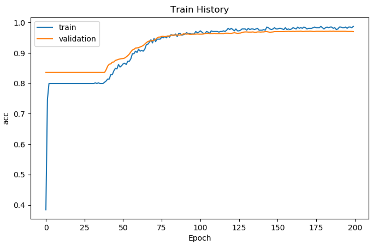
Accuracy Plot – Artificial Intelligence With Python – Edureka

# Display the loss curves for training and validation sets
show_train_history(train_history, 'loss', 'val_loss')

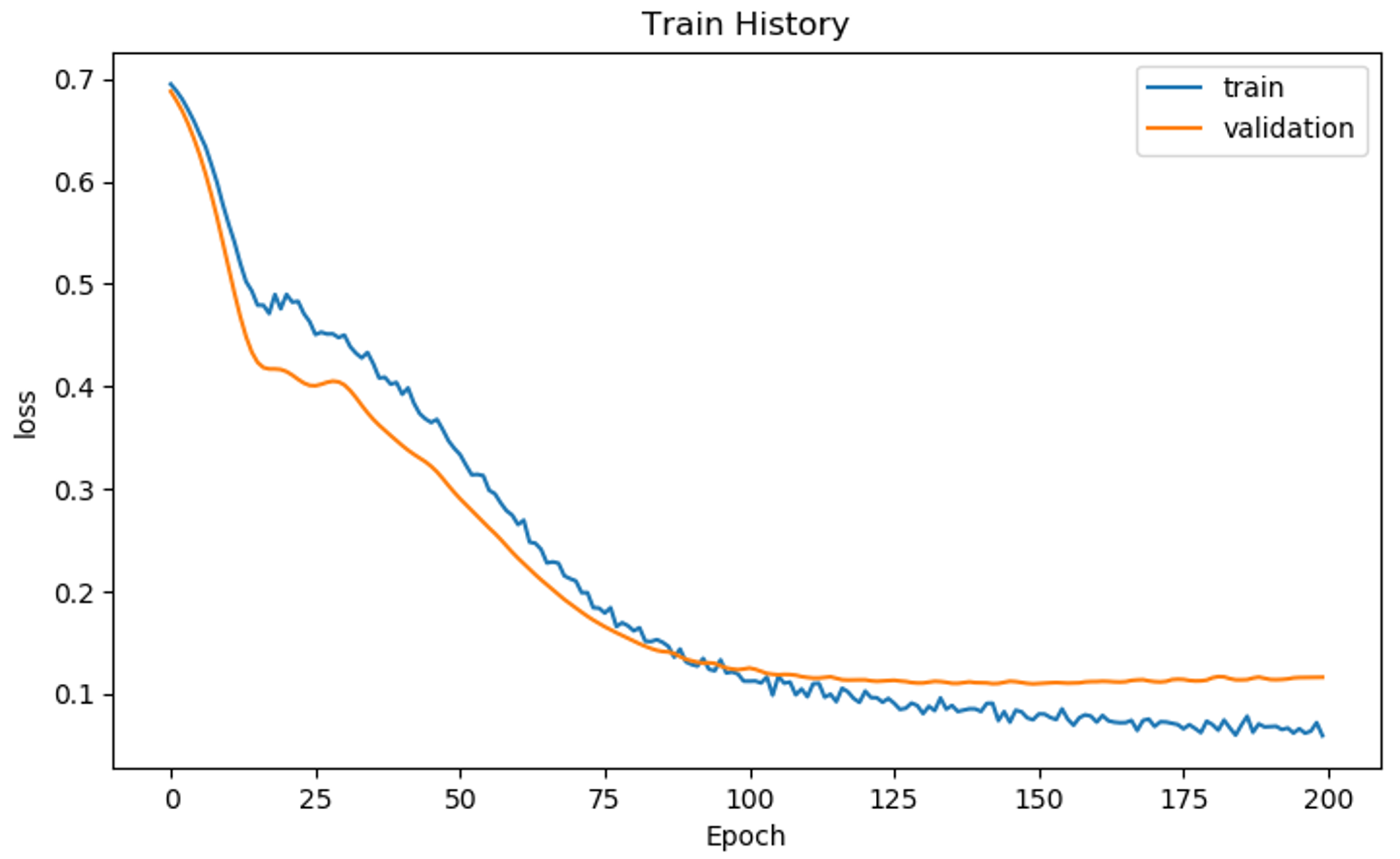
Loss Plot – Artificial Intelligence With Python – Edureka

Step 7: Model Evaluation

# Testing set for model evaluation
scores = model.evaluate(test_feature_trans, test_label)

# Display accuracy of the model
print('n')
print('Accuracy=', scores[1])

Accuracy= 0.98

prediction = model.predict_classes(test_feature_trans)

df_ans = pd.DataFrame({'Real Class': test_label})
df_ans['Prediction'] = prediction

df_ans['Prediction'].value_counts()

df_ans['Real Class'].value_counts()

cols = ['Real_Class_1', 'Real_Class_0'] # Gold standard
rows = ['Prediction_1', 'Prediction_0'] # Diagnostic tool (our prediction)

B1P1 = len(df_ans[(df_ans['Prediction'] == df_ans['Real Class']) & (df_ans['Real Class'] == 1)])
B1P0 = len(df_ans[(df_ans['Prediction'] != df_ans['Real Class']) & (df_ans['Real Class'] == 1)])
B0P1 = len(df_ans[(df_ans['Prediction'] != df_ans['Real Class']) & (df_ans['Real Class'] == 0)])
B0P0 = len(df_ans[(df_ans['Prediction'] == df_ans['Real Class']) & (df_ans['Real Class'] == 0)])

conf = np.array([[B1P1, B0P1], [B1P0, B0P0]])
df_cm = pd.DataFrame(conf, columns=[i for i in cols], index=[i for i in rows])
f, ax = plt.subplots(figsize=(5, 5))
sns.heatmap(df_cm, annot=True, ax=ax, fmt='d')
plt.show()

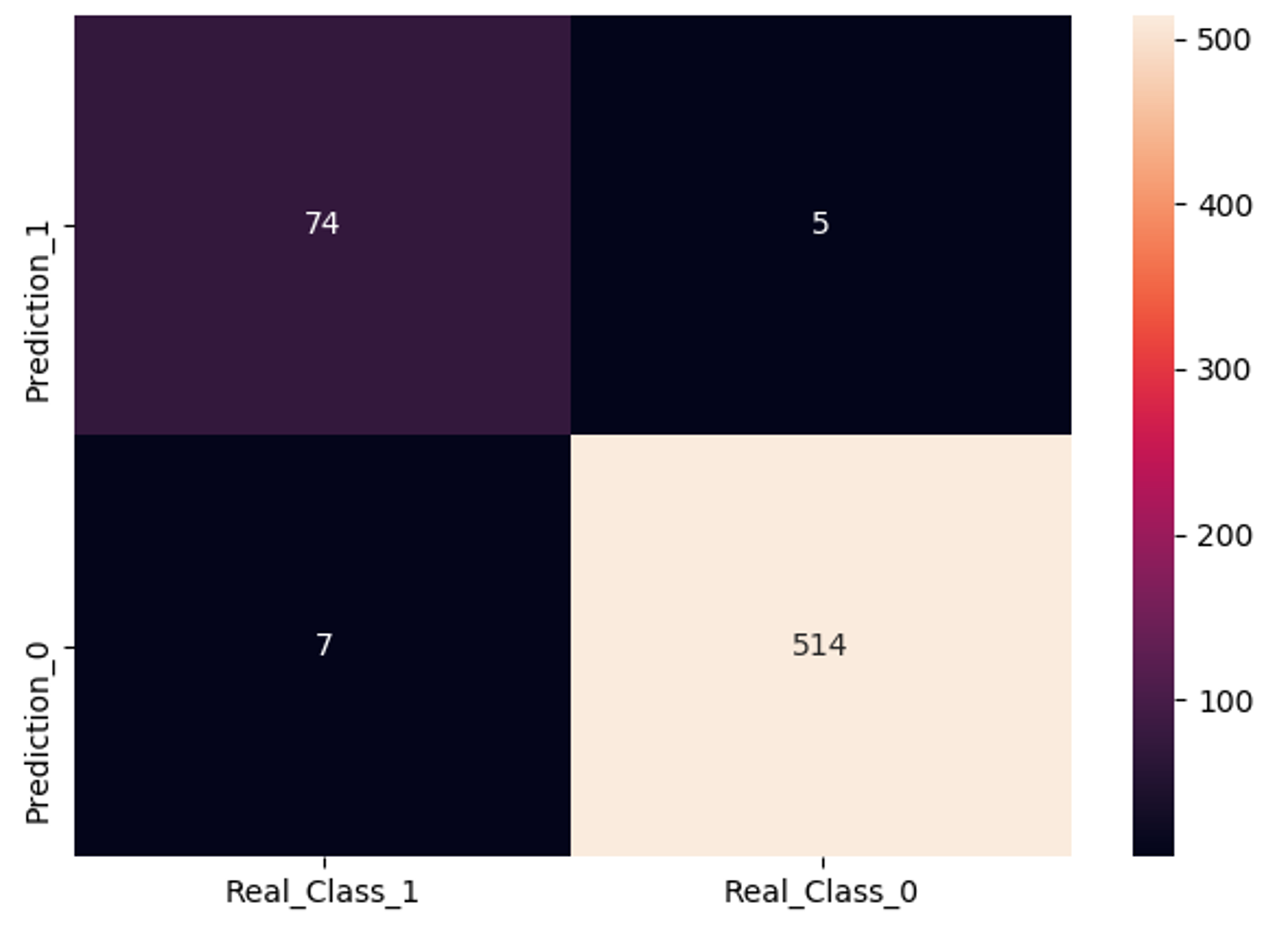
Heatmap – Artificial Intelligence With Python – Edureka

# Making x label be on top is common in textbooks.
ax.xaxis.set_ticks_position('top')

print('Total number of test cases: ', np.sum(conf))

Total number of test cases: 600

# Model summary function
def model_efficacy(conf):
total_num = np.sum(conf)
sen = conf[0][0] / (conf[0][0] + conf[1][0])
spe = conf[1][1] / (conf[1][0] + conf[1][1])
false_positive_rate = conf[0][1] / (conf[0][1] + conf[1][1])
false_negative_rate = conf[1][0] / (conf[0][0] + conf[1][0])

print('Total number of test cases: ', total_num)

Total number of test cases: 600

print('G = gold standard, P = prediction')

# G = gold standard; P = prediction
print('G1P1: ', conf[0][0])
print('G0P1: ', conf[0][1])
print('G1P0: ', conf[1][0])
print('G0P0: ', conf[1][1])
print('--------------------------------------------------')
print('Sensitivity: ', sen)
print('Specificity: ', spe)
print('False_positive_rate: ', false_positive_rate)
print('False_negative_rate: ', false_negative_rate)

Output:

G = gold standard, P = prediction
G1P1: 74
G0P1: 5
G1P0: 7
G0P0: 514
--------------------------------------------------
Sensitivity: 0.9135802469135802
Specificity: 0.9865642994241842
False_positive_rate: 0.009633911368015413
False_negative_rate: 0.08641975308641975

As you can see we’ve achieved an accuracy of 98% which is really good.

So that was all for Deep Learning demo.

Now Let’s focus on the last module where I shall introduce Natural Language Processing.

What Do You Mean By Natural Language Processing?

Natural Language Processing (NLP) is the science of deriving useful insights from natural language text for text analysis and text mining.

NLP uses concepts of computer science and Artificial Intelligence to study the data and derive useful information from it. It is what computers and smartphones use to understand our language, both spoken and written.

Before we understand where NLP is used let me clear out a common misconception. People often tend to get confused between Text Mining and NLP.

Get started with Edureka’s Artificial Intelligence For Beginners Course – a meticulously crafted program that will equip you with cutting-edge insights, strategies, and techniques to reshape your career path in AI. It will empower you to reshape your career path. Seize the opportunity and propel your journey in Artificial Intelligence today!

What Is The Difference Between Text Mining and NLP?

Therefore, we can say that Text Mining can be carried out by using various NLP methodologies.

Now let’s understand where NLP is used.

Natural Language Processing Applications

Here’s a list of real-world applications that make use of NLP techniques:

• Sentimental Analysis: By implementing NLP Tech giants such as Amazon and Netflix, gain insights on their customers to enhance their products and make better recommendations.
• Chatbot: Chatbots are becoming popular in the field of customer service. A popular example is Eva the HDFC chatbot who has addressed over 3 million customer queries, interacted with over half a million unique users, and held over a million conversations.
• Speech Recognition: NLP has been used widely in speech recognition, we’re all aware of Alexa, Siri, Google assistant, and Cortana. They’re all applications of NLP.
• Machine Translation: The popular Google translator uses Natural Language Processing to process and translate one language to the other. It is also used in spell checkers, keyword search, information extraction.
• Advertisement Matching: NLP is also used in advertisement matching to recommend ads based on search history.

Now let’s understand the important concepts in NLP.

Terminologies In Natural Language Processing 

In this section, I will cover all the basic terminologies under NLP. The following processes are used to analyze natural language in order to derive some meaningful insights:

Tokenization

Tokenization basically means breaking down data into smaller chunks or tokens, so that they can be easily analyzed.

For example, the sentence ‘Tokens are simple’ can be broken down into the following tokens:

1. Tokens
2. Are
3. Simple

By performing tokenization you can understand the importance of each token in a sentence.

Stemming

Stemming is the process of cutting off the prefixes and suffixes of the word and taking into account only the root word.

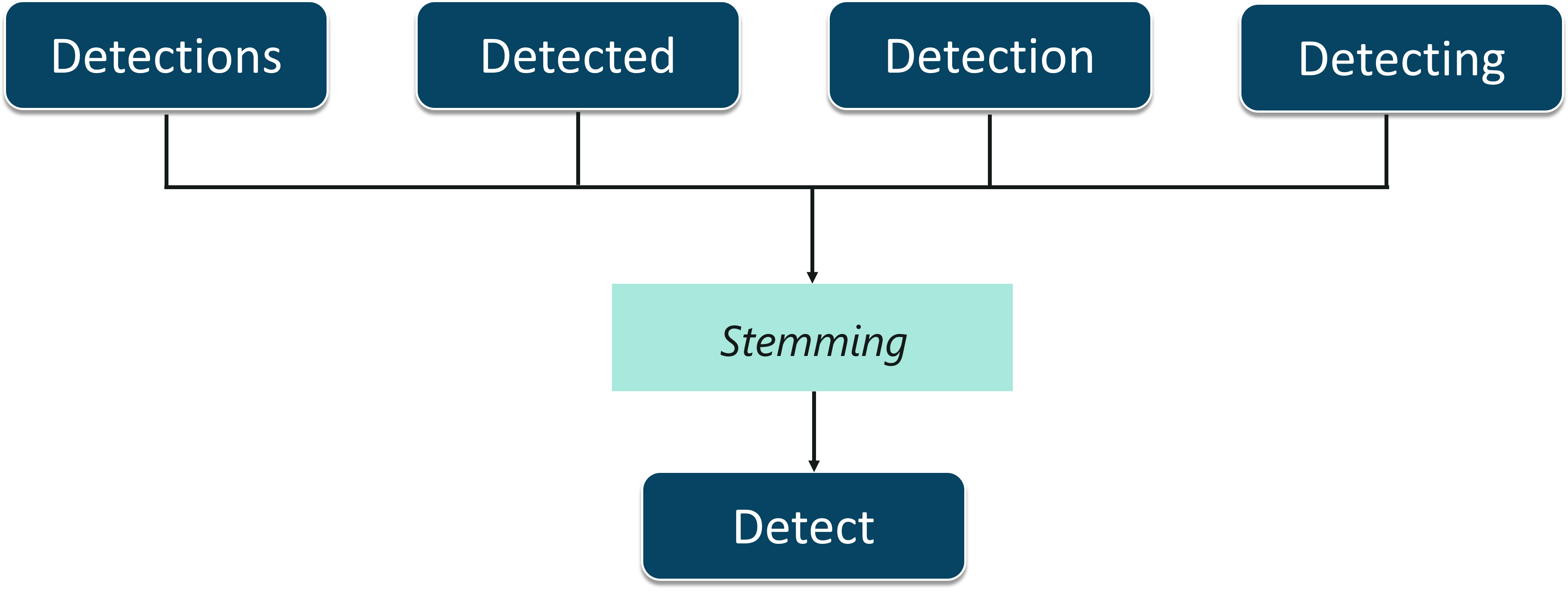
Stemming – Artificial Intelligence With Python – Edureka

Let’s understand this with an example. As shown in the figure, the words,

1. Detection
2. Detecting
3. Detected
4. Detections

can all be trimmed down to their root word, i.e. Detect. Stemming helps in editing such words so that analyzing a document becomes simpler. However, this process can be successful on some occasions. Therefore, another process called Lemmatization is used.

Lemmatization

Lemmatization is similar to stemming, however, it is more effective because it takes into consideration the morphological analysis of the words. The output of lemmatization is a proper word.

An example of Lemmatization is, the words, ‘gone’, ‘going’, and ‘went’ are rooted down to the word ‘go’ by using lemmatization.

Stop Words

Stop words are a set of commonly used words in any language. Stop words are critical for text analysis and must be removed in order to better understand any document. The logic is that if commonly used words are removed from a document then we can focus on the most important words.

Stop Words – Artificial Intelligence With Python – Edureka

For example, let’s say that you want to make a strawberry milkshake. If you open google and type ‘how to make a strawberry milkshake’ you will get results for ‘how’ ‘to’ ‘make’ ‘a’ ‘strawberry’ ‘milkshake’. Even though you only want results for a strawberry milkshake. These words are called stop words. It’s always best to get rid of such words before performing any analysis.

If you want to learn more about Natural Language Processing, you can watch this video by our NLP experts.

So with this, we come to an end of this Artificial Intelligence With Python Blog. If you wish to learn more about Artificial Intelligence, you can give these blogs a read:

1. Artificial Intelligence – What It Is And How Is It Useful?
2. Artificial Intelligence Tutorial: All you need to know about AI
3. AI vs Machine Learning vs Deep Learning
4. Top 10 Benefits Of Artificial Intelligence
5. AI Applications: Top 10 Real World Artificial Intelligence Applications

If you wish to enroll for a complete course on Artificial Intelligence and Machine Learning, Edureka has a specially curated Machine Learning engineer course that will make you proficient in techniques like Supervised Learning, Unsupervised Learning, and Natural Language Processing. It includes training on the latest advancements and technical approaches in Artificial Intelligence & Machine Learning such as Deep Learning, Graphical Models and Reinforcement Learning.

Also, Elevate your skills and unlock the future of technology with our Prompt Engineering Certification! Dive into the world of creativity, innovation, and intelligence. Harness the power of algorithms to generate unique solutions. Don’t miss out on this opportunity to shape the future – enroll now and become a trailblazer in Generative AI. Your journey to cutting-edge proficiency begins here!