


It’s really nice to manage huge data with just a few mouse clicks and Excel is definitely the one tool that will allow you to do this. In case you are still unaware of the magical tricks of Excel, here is an Advanced Excel tutorial to help you learn Excel in great depth.
Take a look at all the topics that are discussed in this article:
So, here is the first and the most important aspect that you need to know in this Advanced Excel Tutorial.
Security
Excel provides security at 3 levels:
- File-level
- Worksheet-level
- Workbook-level
File-level Security:
File-level security refers to securing your Excel file by making use of a password so as to prevent others from opening and modifying it. In order to protect an Excel file, follow the given steps:
1: Click on the File tab
2: Select the Info option
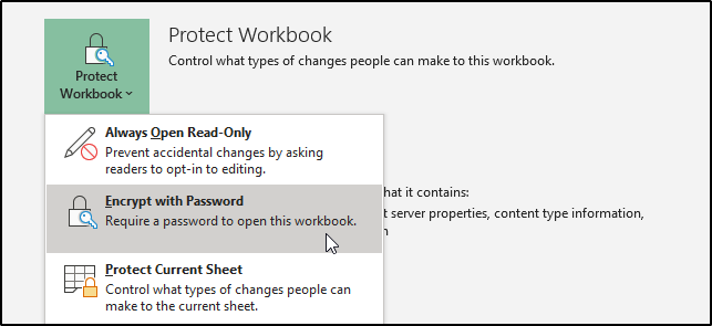
3: Select Protect Workbook option
4: From the list, select Encrypt with Password option

5: Enter a password in the dialog box that appears
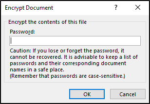

6: Re-enter the password and then, click on OK
Keep the following points in mind while entering passwords:
- Do not forget your password as there is no password recovery available in Excel
- No restrictions are levied but, Excel passwords are case-sensitive
- Avoid distributing password protected files with sensitive information such as bank details
- Protecting a file with a password will not necessarily protect against malicious activities
- Avoid sharing your passwords
Worksheet-level Security:
To protect the data present in a worksheet from being modified, you can lock the cells and then protect your worksheet. Not just this, you can also selectively allow or disallow access to particular cells of your sheet to various users. For example, if you have a sheet that contains details of the sales for different products, and every product is handled by different individuals. you can allow each sales staff to modify the details of only that product which he is responsible for and not the others.
To protect your worksheet you must follow 2 steps:
1: Unlock cells that can be edited by the users
- In the sheet that you wish to protect, select all cells that can be edited by the users
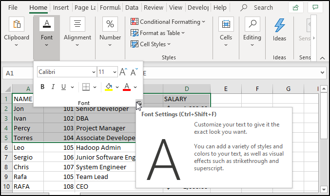
- Open the Font window present in the Home tab
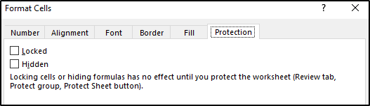
- Select Protection
- Uncheck the Locked option


2: Protecting the worksheet
- To protect the sheet, click on the Review tab and then select the Protect Sheet option
- You will see the following dialog box
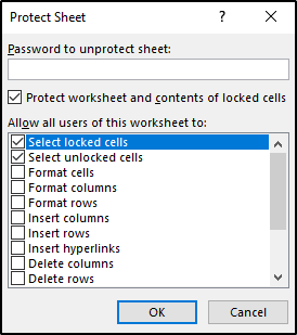

- From the “Allow all users of this worksheet to” option, select any of the elements that you wish to
- Give some password of your choice and click on OK (The setting of a password is optional)
Unportecting a Worksheet:
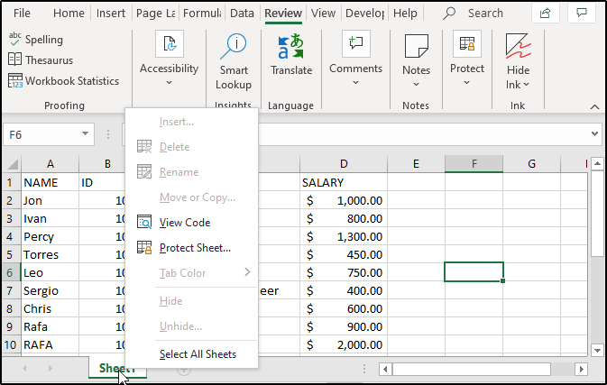
In case you want to unprotect the sheet, you can do it by selecting the Unprotect Worksheet option from the Review tab. In case you have specified any password while protecting the sheet, Excel will ask you to enter the same in order to unprotect the sheet.
Workbook-level Security:
Workbook-level security will help you prevent other users from adding, deleting, hiding, or renaming your sheets. Here is how you can protect your workbooks in Excel:
1: From the Review tab, select Protect Workbook option, you will see the following dialog box:
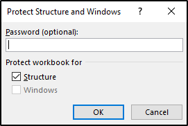

2: Enter some password of your choice and click on OK (This is optional, if you do not enter any password, anyone can unprotect your workbook)
3: Re-enter the password and click on OK
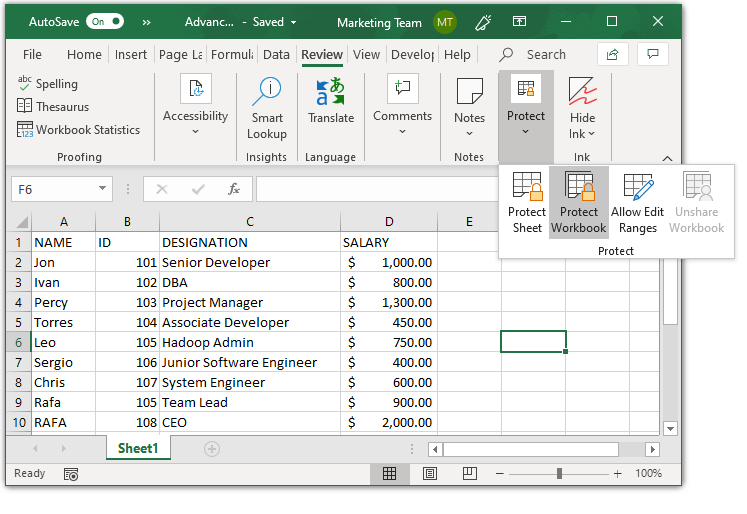
When your workbook is protected, you will see that the Protect Workbook option will be highlighted as shown below:


MS Excel Themes
MS Excel provides a number of document themes to help you create formal documents. Using these themes, it will be very easy for you to harmonize different fonts, colors or graphics. You also have an option to either change the complete theme or just the colors or fonts, etc according to your choice. IN Excel, you can:
- Make use of standard color themes
- Create your theme
- Modify the font of themes
- Change effects
- Save your customized theme
Make use of standard color themes:
In order to choose a standard theme, you can do as follows:
- Select the Page Layout tab from the Ribbon
- From the Themes group, click on Colors
- Select any color of your choice
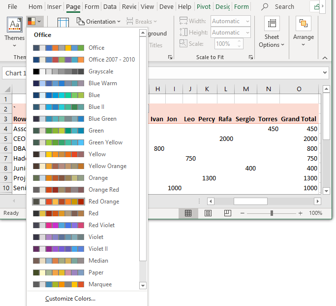

The first group of colors that you see. are the default MS Excel colors.
Create your theme:
In case you want to customize your own colors, click on Customize Colors option present at the end of the dropdown list shown in the image above, and you will see a dialog box as shown in the image below:
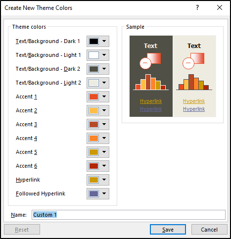

From the above dialog box, select any color of your choice for the Accents, Hyperlinks, etc. You can also create your own color by clicking on the more colors option. You will be able to see all the changes you make in the Sample pane present at the right side of the dialog box shown in the image above. Not just this, you can also give a name to the theme you create in the Name box and Save it. In case you do not want to save any of the changes you made, click on Reset and then click on Save.
Modify the font of themes:
Just like how you could change the theme colors, Excel allows you to change the font of themes. This can be done as follows:
- Click on Page Layout from the Ribbon tab
- Open the dropdown list of Fonts
- Select any font style you like
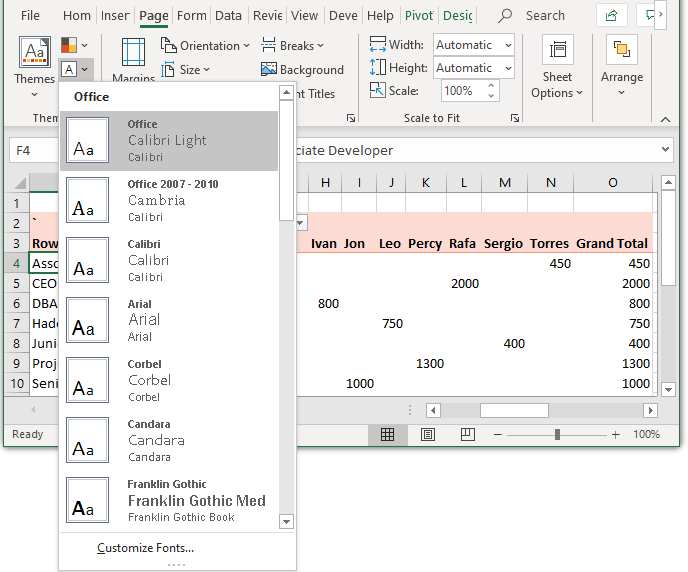

You can also customize your own font styles by clicking on the Customize Fonts option. you will the following dialog box opening when you click on it:
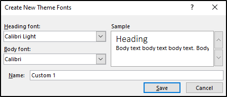
Give any Heading and Body font of your choice and then, give it a name. Once this is done, click on Save.

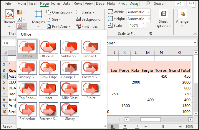
Change Effects:
Excel provides a huge set of theme effects such as lines, shadows, reflections, etc that you can add on. To add effects, click on Page Layout and open the Effects dropdown list from the Themes group then select any effect you wish to.
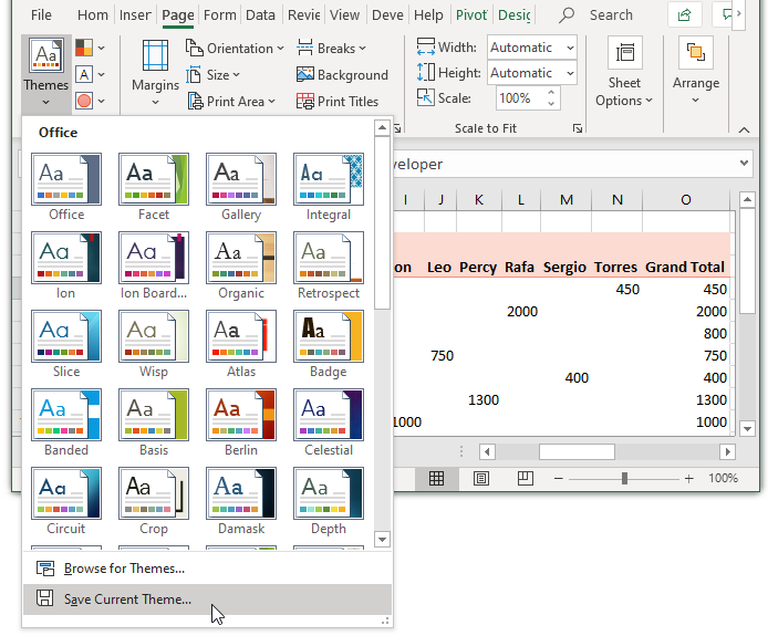
Save your customized theme:

You can save all the changes you make by Saving the current theme as follows:
1: Click on Page Layout, select Themes
2: Choose the Save Current Theme option
3: Give a name to your theme in the Name box
4: Click Save

Note: The theme that you Save will be saved in the Document Themes folder on your local drive in the .thmx format.
Templates
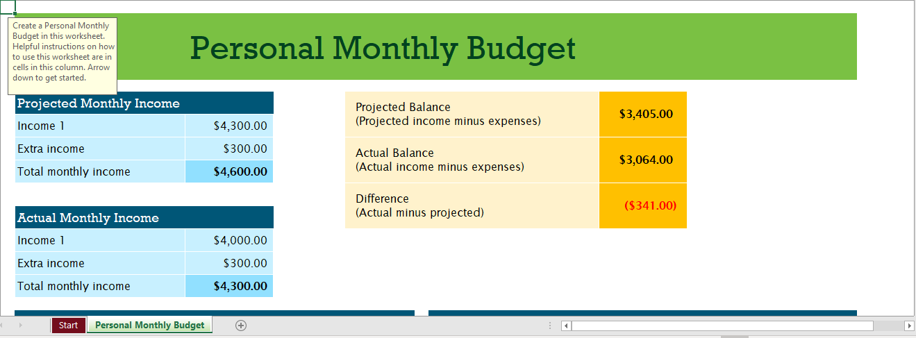
A Template, in general, is a pattern or a model that forms the base of something. Excel templates help you increase your production rates as they help you save time and effort to create your documents. In order to make use of Excel templates, you should click on File, then select New. Here, you will be able to see a number of Excel templates that you can choose for any type of document such as Calenders, Weekly attendance reports, Simple invoices, etc. You can also look for a template online. For example, if you choose the Personal Monthly Budget template, your template will look as shown in the image below:

Graphics
Unlike what many people think, Excel does not just allow you to play around with data, but it also allows you to add graphics to it. To add graphics, click on the Insert tab and you will be able to see a number of options such as adding images, shapes, PivotTables, Pivot Charts, Maps, etc.
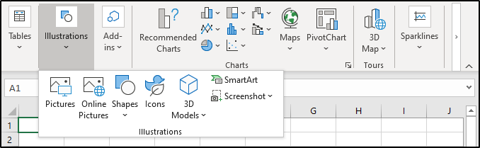
Inserting Images:
In this Advanced Excel tutorial, I will show you all how to add images to your Excel documents. First, click on Insert and then open the Illustrations list, select Pictures.

Select any picture you wish to add to your document. In the image shown below, I have added the logo of Excel:

Similarly, you can also add shapes, icons, SmartArt, etc to your documents.
Printing Options:
To print your MS Excel Worksheets, click on File and then select the Print option. You will see a number of options before printing the document that allows you to print your document in different patterns and layouts. You can change page orientations, add margins, change printers, etc.
Data Tables
Data tables in Excel are created to experiment with different values for a formula. You can create either one or two variable Data tables in Excel. Data tables are one of the three types of What-if analysis tools available in Excel.
In this Advanced Excel Tutorial, I will be showing you all how to create both one-variable and two-variable Data tables.
Creating a One-Variable Data Table:
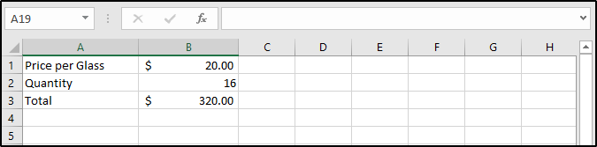
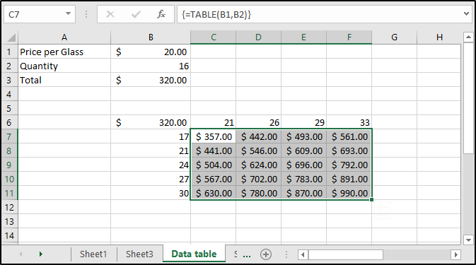
Say for example you purchased 16 glasses at the rate of $20 each. This way, you will have to pay a total of $320 for 16 glasses respectively. Now, in case you want to create a data table that will show you the prices for different quantities of the same item, you can do as follows:
1: Set up the data as follows:

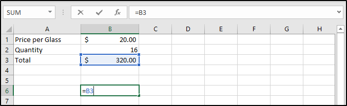
2: Then, copy the result present in B3 to another cell

3: Write down different quantities of items as shown below:
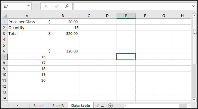

4: Select the newly created range, click on the Data tab, select What-If Analysis from the Forecast group. Then select the Data Table option.
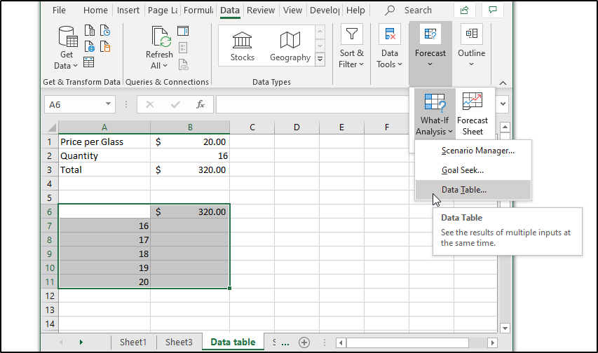

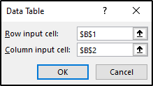
5: From the dialog box shown below, specify the column input cell. (This is because the new quantities are specified in columns)
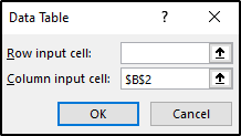

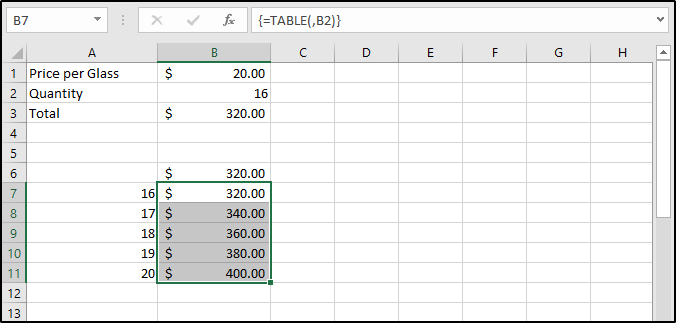
6: Once this is done, you will see all the resultant values. Select all cells with the output values and specify the $ symbol to them:

Two-variable Data Table:
To create a two-variable Data Table for the same data that was taken in the previous example, follow the given steps:
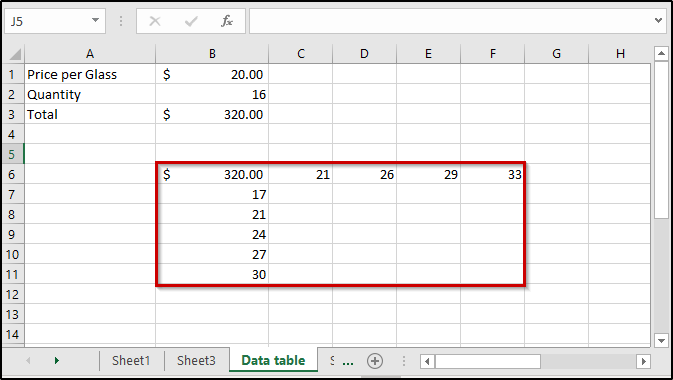
1: Copy the result present in B3 to some cell and specify test row and column values as shown below:

1: Select the range, click on the Data tab
2: Select What-If analysis from the Forecast group
3: In the window that appears, enter the Row and the Column input cell as shown below:

4: Once you click OK, you will see the result for the complete table
5: Select all the output cells, and then specify the $ symbol

Charts
Charts give graphical representation to your data. These charts visualize numerical values in a very meaningful and easy-to-understand manner. Charts are a very essential part of Excel and they improved greatly with every new version of MS Excel. There are many types of Charts that you can use such as Bar, Line, Pie, Area, etc.
This Advanced Excel tutorial will help you learn how to create charts in Excel.
Creating Charts:
To insert a chart, follow the given steps:
1: Prepare your chart data

2: Select the prepared data, click on Insert present in the Ribbon tab
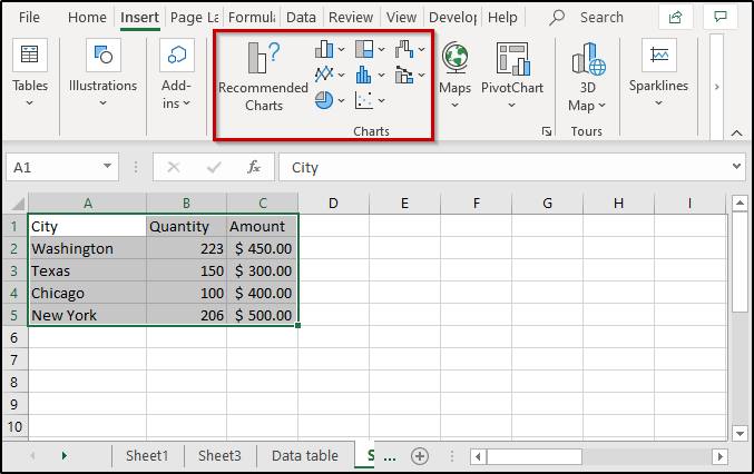

3: From the Charts group, select any chart of your choice

Pivot Tables:
Excel Pivot Tables are statistical tables that condense the data of tables having extensive information. These tables help you visualize your data based on any of the fields present in your data table. Using Pivot Tables, you can visualize your data by changing the fields’ rows and columns, add filters, sorting your data, etc.
Creating Pivot tables: To create a pivot table, follow the given steps:
1: Select the rage for which you want to create a pivot table
2: Click on Insert
3: Select Pivot Table from the Tables group

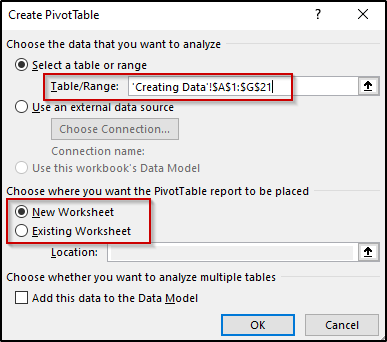
4: Check if the given range is correct
5: Select the place where you want to create the table i.e New Worksheet or the same
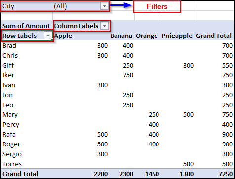
6: Excel will create an empty Pivot Table


7: Drag and drop fields you wish to add in order to customize your pivot table


You will see the following table is created:

Pivot Charts
Excel Pivot Charts are built-in visualization tools for Pivot tables. Pivot Charts can be created as follows;
1: Create the Pivot Table

2: Click on the Insert tab
3: Select Pivot Charts from the Charts group
4: This will open up a window that will show you all the available Pivot Charts
5: Select any type graph and click on OK
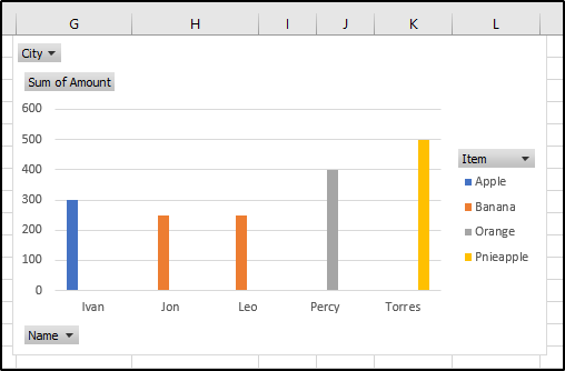

As you can see, a Pivot Chart has been created for my Pivot Table.
Data Validation
One of the most important topics of this Advanced Excel Tutorial is Data Validation. This feature, as the name suggests, allows you to configure the cells of your Excel Worksheets to accept some particular type of data. For example, if you want a certain number of cells in your sheet and you want them to accept only dates, you can do it easily using the Data Validation feature of Excel. In order to do this, follow the given steps:
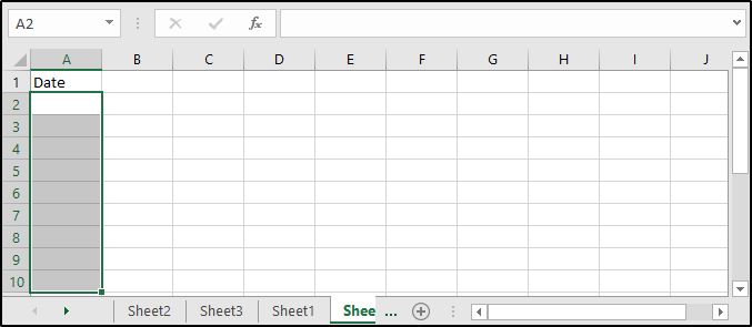
1: Select all the cells that you wish to assign a particular data type to:

2: Click on the Data tab present in the Ribbon
3: From the Data Tools group, select Data Validation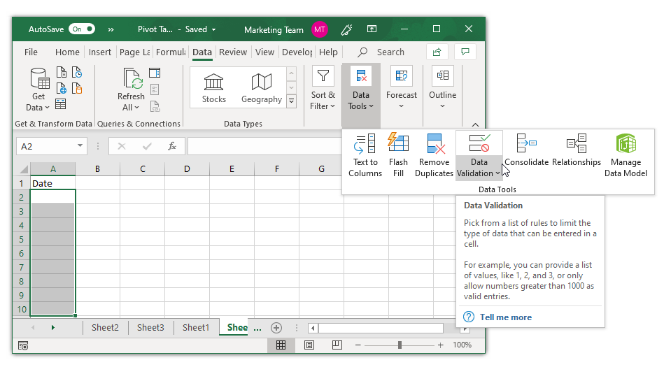

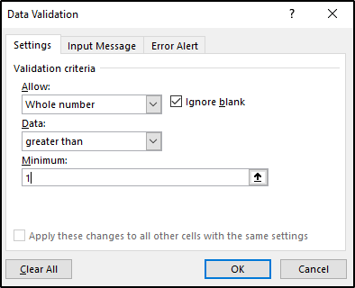
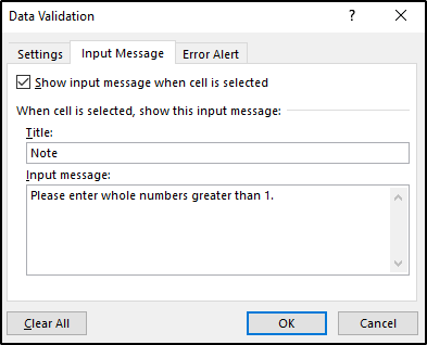
4: You will see a popup window with three options i.e Settings, Input Message, and Error Alert
- Settings will allow you to choose any type of data that you want the selected range to accept
- The Input Message section will allow you to enter a message for the user giving him some details regarding the acceptable data
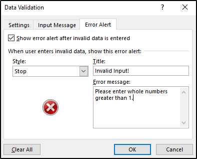
- The Error Message section will inform the user that he has made some mistake in giving the desired input
- Settings will allow you to choose any type of data that you want the selected range to accept


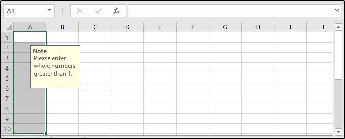
Now, if you select any cell in the selected range, you will first see a message asking the user to enter whole numbers greater than 1.

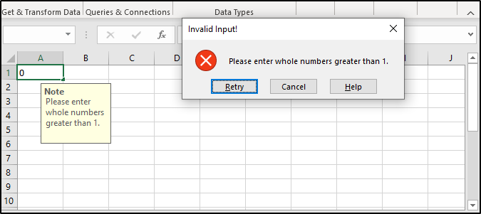
In case the user fails to do so, he will see an appropriate error message as shown below:

Data Filtering
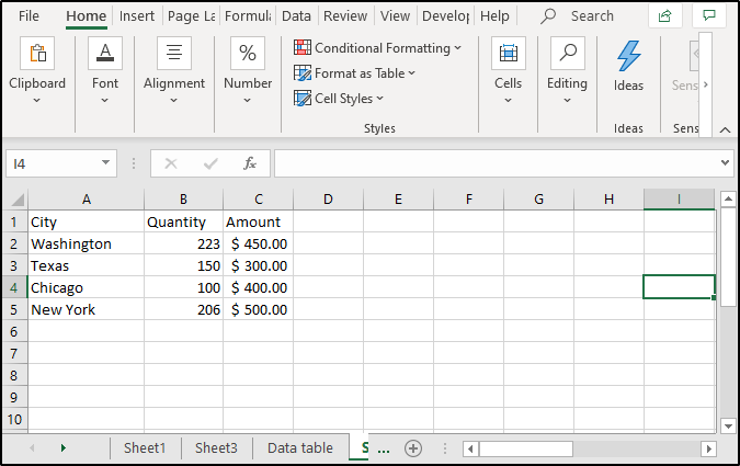
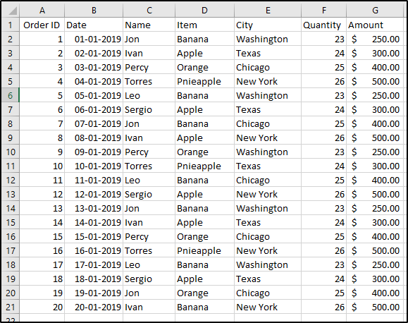
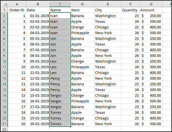
Filtering data refers to fetching some particular data that meets some given criteria. Here is the table that I will be using to filter out data:

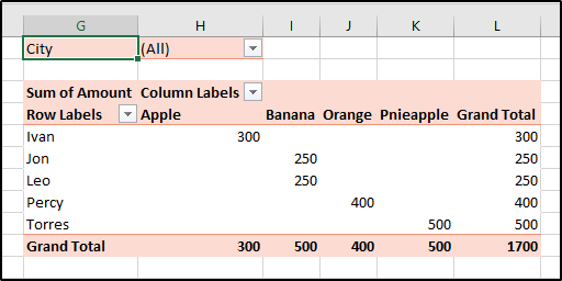
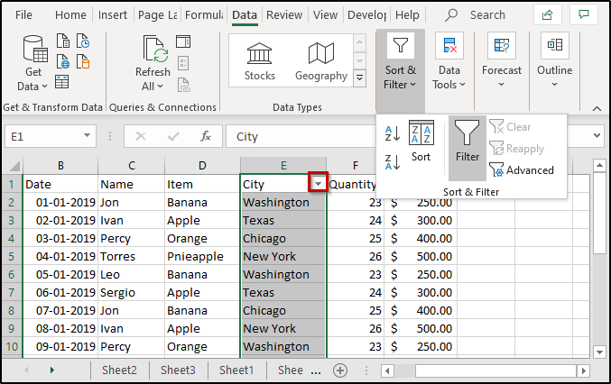
Now, in case you want to filter out the data just for New York, all you have to do is select the City column, click on Data present in the Ribbon tab. Then, from the Sort&Filter group, select Filter.
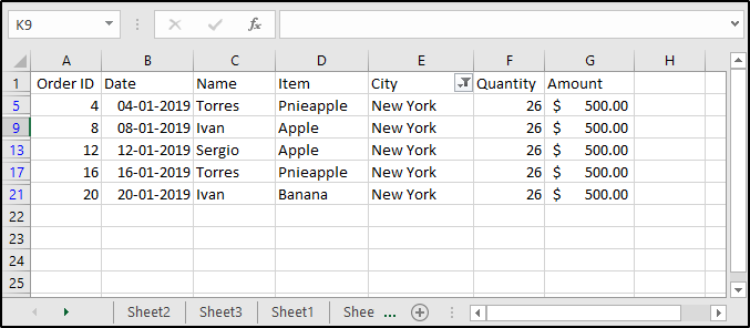
Once this is done, the City column shows a dropdown list that holds the names of all the cities. To filter the data for New York, open the dropdown list, unselect the Selected All option and check New York and then click on OK. You will see the following filtered table:

Similarly, you can also apply multiple filters by just selecting the range you want to apply the filter to, and then selecting the Filter command.
Learn How do you use an advanced filter to filter by date in Excel?
Sorting
Data sorting in Excel refers to arranging the data rows on the basis of data present in the columns. For example, you can rearrange the names from A-Z or arrange numbers from ascending or descending orders respectively.
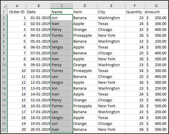
For instance, consider the table shown in the previous example. If you want to rearrange the names of the vendors starting from A, you can do as follows:
- Select all the cell you want to sort

- Click on Sort present in the Data tab and you will see a dialog box as shown below:
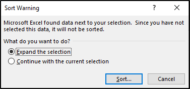

- Here, you have two options based on your wish to Expand your selection for the complete data or only for the current selection (I’m choosing the 2nd option)
- Once that is done, you will see the following dialog box:
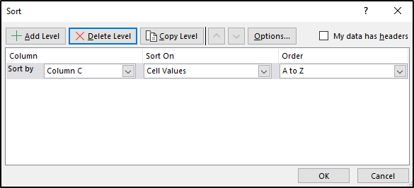

- Here, you can add more columns, delete columns, change the order, etc. Since I want to sort the column from A-Z, I will click on OK.
Here is what the table looks like:

Similarly, you can sort your table using multiple levels and orders.
Cross Referencing in MS Excel
In case you want to look for data across multiple sheets in your workbook, you can make use of the VLOOKUP function. The VLOOKUP function in Excel is used to look up and bring forth required data from spreadsheets. V in VLOOKUP refers to Vertical and if you want to use this function, your data must be organized vertically. For a detailed explanation on VLOOKUP.
Using VLOOKUP to fetch data from multiple sheets:
In order to use the VLOOKUP function to fetch values present in different sheets, you can do as follows:
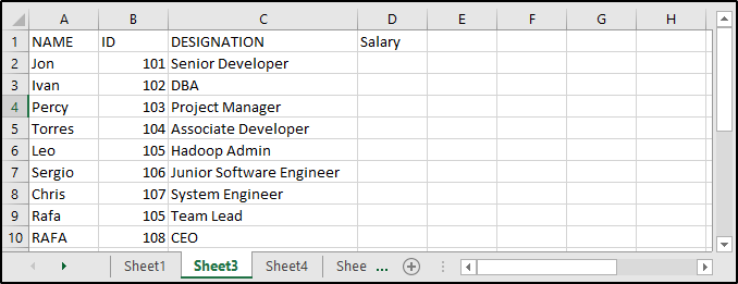
Prepare the data of bo the sheets as shown:
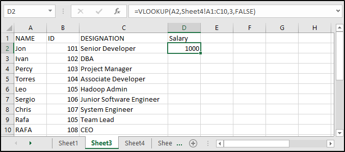
Sheet3:

Sheet4:
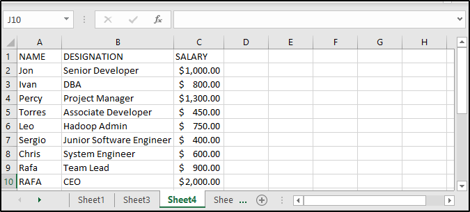

Now, in order to fetch the salaries of these employees from sheet4 to sheet3, you can use VLOOKUP as follows:
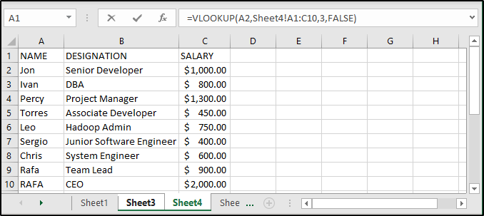

You can see that both sheet3 and sheet4 are selected. When you execute this command, you will get the following result:

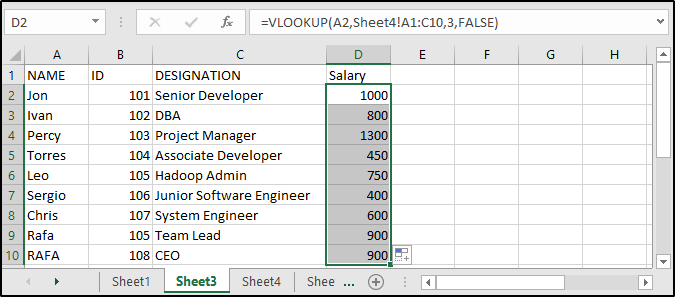
Now, to fetch the salaries of all the employees, just copy the formula as shown below:

Macros
Macros are a must to be learnt in Excel. Using these Macros, you can automate the tasks that you perform regularly by just recording them as macros. A macro in Excel is basically an action or set actions that can be performed again and again automatically.
In this Advanced MS Excel Tutorial, you will be learning how you can create and make use of macros.
Creating a Macro:
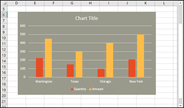
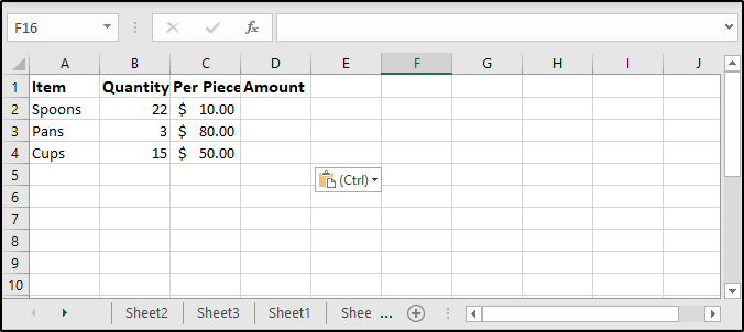
In the following example, I have some information regarding a store and I will create a macro in order to create a data graph for the sales of the items along with their amounts and quantities.
- First, create the table as shown below:

- Now, click on the View tab
- Click on Macros and select the Record Macro option
- Enter some name for the macro you are going to create in the dialog box that appears and if you want, you can also create a shortcut for this macro
- Next, click on OK (Once this is done, Excel starts to record your actions)
- Select the first cell under the Amount column
- Type “=PRODUCT(B2, B3)” and hit enter
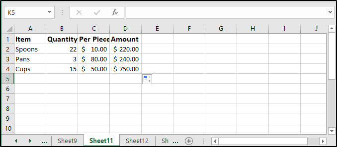
- Insert a $ sign from the Home tab Numbers group
- Then, copy the formula to the rest of the cells

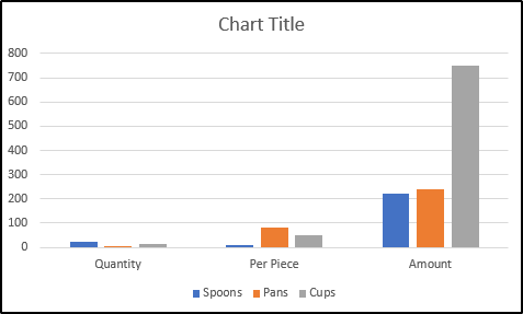
- Now, click on Insert and choose any chart you prefer. Here is what the chart for the table shown in the image above looks like:

- Once the actions are completed, click on View and select Stop Recording option from Macros
When you do this, your macro will be recorded. Now every time you wish to perform all these actions, simply run the macro and you will be able to see the outputs accordingly. Also, make a note that each time you make changes to the values present in the cells, your macro will make changes accordingly when you run it and will show the updated results automatically.
Language Translation
Excel brilliantly allows users to translate the data into different languages. It can auto-detect the language present in your data and then convert it into any desired language that is present in Excel’s list of languages. Follow the given steps to perform language translation:
- Click on the Review tab
- Select Translate from Language group
- You will see a Translator window where you can either let Excel detect the language present in the sheet or give some specific language
- Then, from the ‘To‘ dropdown list, select any language you wish to convert the data into


As you can see, the text that I have has been converted to Hindi.
This brings us to the end of this article on Advanced Excel Tutorial. I hope you are clear with all that has been shared with you. Make sure you practice as much as possible and revert your experience.
Got a question for us? Please mention it in the comments section of this “Advanced Excel Tutorial” blog and we will get back to you as soon as possible.
To get in-depth knowledge on any trending technologies along with their various applications, you can enroll for live Edureka MS Excel Online training with 24/7 support and lifetime access.
Also Read:
Count Specific Characters in Google Sheets How to count specific characters in google sheets?